Mathematical Foundation of Reinforcement Learning-Concept Notes

Reference Sources:

1. Shiyu Zhao. 《Mathematical Foundation of Reinforcement Learning》Chapter 1-3.
2. OpenAI Spinning Up
3. Lu yukuan’s notes

1. Basic Concepts

1.1 A grid world example (Consistent example)

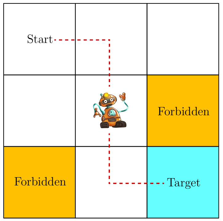
Consider an example as shown in Figure, where a robot moves in a grid world. The robot, called agent, can move across adjacent cells in the grid. At each time step, it can only occupy a single cell.The white cells are accessible for entry, and the orange cells are forbidden . There is a target cell that the robot would like to reach. We will use such grid world examples throughout RL since they are intuitive for illustrating new concepts and algorithms.

How can the goodness of a policy be defined? The idea is that the agent should reach the target without entering any forbidden cells, taking unnecessary detours, or colliding with the boundary of the grid.It would be trivial to plan a path to reach the target cell if the agent knew the map of the grid world.The task becomes nontrivial if the agent does not know any information about the environment in advance. Then, the agent must interact with the environment to find a good policy by trial and error. To do that, the concepts presented in the rest of the chapter are necessary.

1.2 State and action ( $ s_n, a_m $ )

State describes the agent’s status with respect to the environment. The set of all the states is called the state space, denoted as $\mathcal{S}=\left\{s_1,s_2, \ldots, s_n\right\}$.

For each state, the agent can take actions $\mathcal{A}$. Different states can have different action spaces ($\mathcal{A}(s)$ when at state $s$) . The set of all actions is called the action space, denoted as $\mathcal{A}=\left\{a_1, a_2,\ldots, a_m\right\}$.

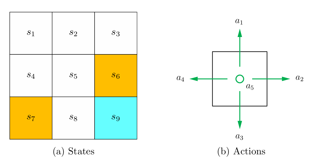
In this RL serie, we consider the most general case: $\mathcal{A}\left(s_i\right)=\mathcal{A}=\left\{a_1, \ldots, a_5\right\}$ for all $i$.

1.3 States and Observations

You may see the terminology “observation”. It’s similar to “states”. Whatt’s the difference?

• A state $s$ is a complete description of the state of the world. There is no information about the world which is hidden from the state.

• An observation $o$ is a partial description of a state, which may omit information.

• The environment is fully observed when the agent is able to observe the complete state of the environment.

• The environment is partially observed when the agent can only see a partial observation.

Reinforcement learning notation sometimes puts the symbol for state ($s$), in places where it would be technically more appropriate to write the symbol for observation($o$).

Specifically, this happens when talking about how the agent decides an action: we often signal in notation that the action is conditioned on the state, when in practice, the action is conditioned on the observation because the agent does not have access to the state.

1.4 State transition ( $p(s_{n} \mid s_1, a_{2})=x$ );

When taking an action, the agent may move from one state to another. Such a process is called state transition. For example, if the agent is at state $s_1$ and selects action $a_2$ , then the agent moves to state $s_2$. Such a process can be expressed as

$$s_1 \stackrel{a_2}{\rightarrow} s_2$$

• the agent will be bounced back because it is impossible for the agent to exit the state space. Hence, we have $s_1 \stackrel{a_1}{\rightarrow} s_1$.
• What is the next state when the agent attempts to enter a forbidden cell, for example, taking action $a_2$ at state $s_5$ ? Two different scenarios may be encountered.
• 1. In the first scenario, although $s_6$ is forbidden, it is still accessible. In this case, the next state is $s_6$; hence, the state transition process is $s_5 \stackrel{a_2}{\longrightarrow} s_6$.
• 1. In the second scenario, $s_6$ is not accessible because, for example, it is surrounded by walls. In this case, the agent is bounced back to $s_5$ if it attempts to move rightward; hence, the state transition process is $s_5 \stackrel{a_2}{\rightarrow} s_5$.
• Which scenario should we consider? The answer depends on the physical environment. In this series, we consider the first scenario where the forbidden cells are accessible, although stepping into them may get punished. This scenario is more general and interesting. Moreover, since we are considering a simulation task, we can define the state transition process however we prefer. In real-world applications, the state transition process is determined by real-world dynamics.

Mathematically, the state transition process can be described by conditional probabilities. $p(s_{n} \mid s_1, a_{2})=x , x\in(0,1)$;

1.5 Policy ($\pi(a \mid s)$)

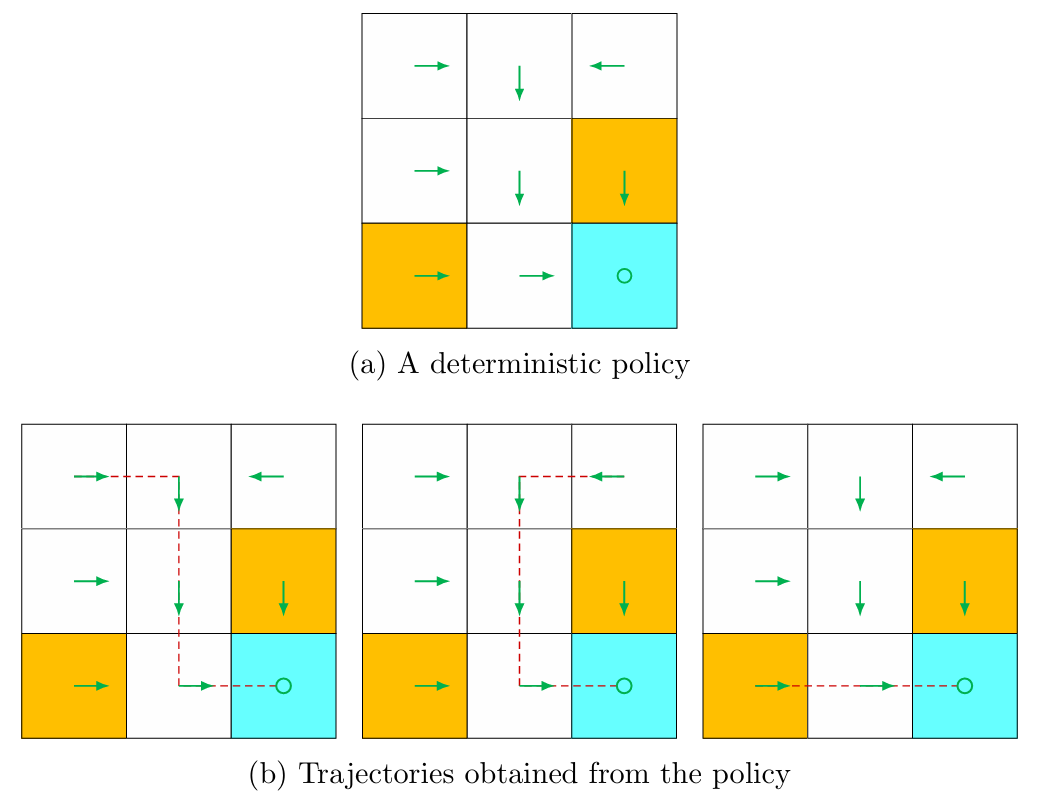
A policy tells the agent which actions to take at every state. Intuitively, policies can be depicted as arrows (see Figure 1.4(a)). Following a policy, the agent can generate a trajectory starting from an initial state (see Figure 1.4(b)).

A policy can be deterministic or stochastic.

1. Deterministic policy
   A deterministic policy is usually denoted by $\mu$ :

   $$a_t=\mu\left(s_t\right) .$$

2. Stochastic policy (conditional probabilities)
   A stochastic policy is usually denoted by $\pi$ :

   $$a_t \sim \pi\left(\cdot \mid s_t\right) .$$

   In this case, at state $s$, the probability of choosing action $a$ is $\pi(a \mid s)$. It holds that $\sum_{a \in \mathcal{A}(s)} \pi(a \mid s)=1$ for any $s \in \mathcal{S}$.

In RL, the policies are often parameterized, the parameters are commonly denoted as $\theta$ or $\phi$ and are written as a subscript on the policy symbol:

$$\begin{aligned} a_t & = \mu_{\theta}(s_t) \\ a_t & \sim \pi_{\theta}(\cdot | s_t). \end{aligned}$$

1.6 Rewards ($r(s, a)$, $p(r \mid s,a)$)

After executing an action at a state, the agent obtains a reward, denoted as $r$, as feedback from the environment. The reward is a function of the state $s$ and action $a$. Hence, it is also denoted as $r(s, a)$. Its value can be a positive or negative real number or zero.

In the grid world example, the rewards are designed as follows:

1. If the agent attempts to exit the boundary, let $r_{\text {boundary }}=-1$.
2. If the agent attempts to enter a forbidden cell, let $r_{\text {forbidden }}=-1$.
3. If the agent reaches the target state, let $r_{\text {target }}=+1$.
4. Otherwise, the agent obtains a reward of $r_{\text {other }}=0$.

A reward can be interpreted as a human-machine interface , with which we can guide the agent to behave as we expect. For example, with the rewards designed above, we can expect that the agent tends to avoid exiting the boundary or stepping into the forbidden cells. Designing appropriate rewards is an important step in reinforcement learning. This step is, however, nontrivial for complex tasks since it may require the user to understand the given problem well. Nevertheless, it may still be much easier than solving the problem with other approaches that require a professional background or a deep understanding of the given problem.

One question that beginners may ask is as follows: if given the table of rewards, can we find good policies by simply selecting the actions with the greatest rewards? The answer is no. That is because these rewards are immediate rewards that can be obtained after taking an action. To determine a good policy, we must consider the total reward obtained in the long run (see Section 1.7 for more information). An action with the greatest immediate reward may not lead to the greatest total reward. It is possible that the immediate reward is negative while the future reward is positive. Thus, which actions to take should be determined by the return (i.e., the total reward) rather than the immediate reward to avoid short-sighted decisions.

1.7 Trajectories and Return

A trajectory $\tau$ is a state-action-reward chain $\tau = (s_1, a_1, s_2, a_2, …)$.

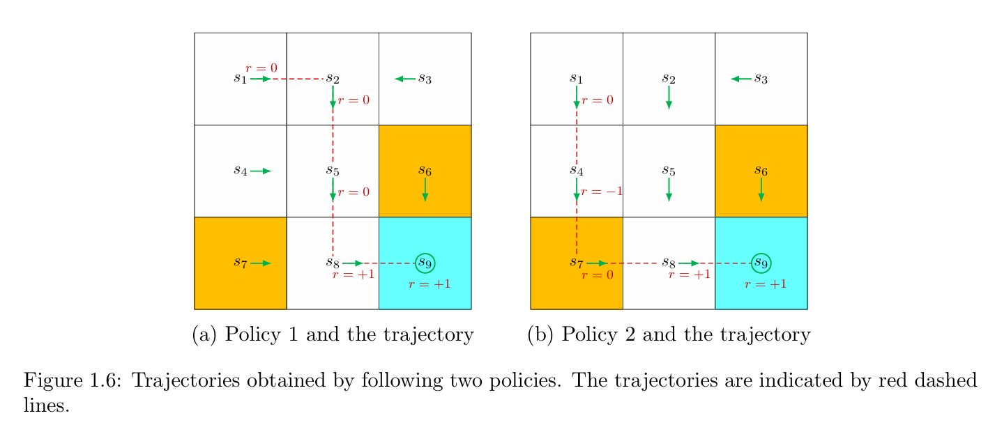
For example, given the policy shown in Figure 1.6(a), if the agent can move along a trajectory as follows:

$$s_1 \underset{r=0}{\stackrel{a_2}{\longrightarrow}} s_2 \underset{r=0}{\stackrel{a_3}{\longrightarrow}} s_5 \underset{r=0}{\stackrel{a_3}{\longrightarrow}} s_8 \underset{r=1}{\stackrel{a_2}{\longrightarrow}} s_9 .$$

The undiscounted return of this trajectory is defined as the sum of all the rewards collected along the trajectory:

$$\text { return }=0+0+0+1=1 .$$

This return is undiscounted. But in RL we usually consider discounted return with a discount rate $\gamma \in (0,1)$ especially for the trajectory of infinite length.

$$\text { return }= 0+ \gamma 0+ \gamma^2 0+ \gamma^3 1 = \gamma^3 .$$

The introduction of the discount rate is useful for the following reasons.

1. it removes the stop criterion and allows for infinitely long trajectories.
2. the discount rate can be used to adjust the emphasis placed on near- or far-future rewards. In particular, if is close to 0, then the agent places more emphasis on rewards obtained in the near future. The resulting policy would be short-sighted. If is close to 1, then the agent places more emphasis on the far future rewards. The resulting policy is far-sighted and dares to take risks of obtaining negative rewards in the near future.

Returns are also called total rewards or cumulative rewards.

1.8 Episodes

When interacting with the environment by following a policy, the agent may stop at some terminal states. In this case, the resulting trajectory is finite, and is called an episode (or a trial, rollout).

However, some tasks may have no terminal states. In this case, the resulting trajectory is infinite.

Tasks with episodes are called episodic tasks. some tasks have no terminal states are called continuing tasks.

In fact, we can treat episodic and continuing tasks in a unified mathematical manner by converting episodic tasks to continuing ones. We have two options:

1. First, if we treat the terminal state as a special state, we can specifically design its action space or state transition so that the agent stays in this state forever. Such states are called absorbing states, meaning that the agent never leaves a state once reached.
2. Second, if we treat the terminal state as a normal state, we can simply set its action space to the same as the other states, and the agent may leave the state and come back again. Since a positive reward of $r=1$ can be obtained every time $s_9$ is reached, the agent will eventually learn to stay at $s_9$ forever (self-circle) to collect more rewards.

In this RL series, we consider the second scenario where the target state is treated as a normal state whose action space is $\mathcal{A}\left(s_9\right)=\left\{a_1, \ldots, a_5\right\}$.

1.9 Markov decision processes

This section presents the basic RL concepts in a more formal way under the framework of Markov decision processes (MDPs).

An MDP is a general framework for describing stochastic dynamical systems. The key ingredients of an MDP are listed below.

Sets:

• — State space: the set of all states, denoted as $\mathcal{S}$.
• — Action space: a set of actions, denoted as $\mathcal{A}(s)$, associated with each state $s \in \mathcal{S}$.
• — Reward set: a set of rewards, denoted as $\mathcal{R}(s, a)$, associated with each state-action pair $(s, a)$.

Note:

1. The state, action, reward at time index $t$ are denoted as $s_t, a_t, r_t$ separately.
2. The reward depends on the state $s$ and action $a$, but not the next state $s^{\prime}$. because since $s^{\prime}$ also depends on $s$ and $a$ i.e. $p(s^{\prime}\mid s,a)$ ($s,a$后下一状态可能是随机的，$s’$代表的下一状态是固定的一种情况，因此与$s’$无关只与$s,a$有关).

Model:

• State transition probability: At state $s$, when taking action $a$, the probability of transitioning to state $s^{\prime}$ is $p\left(s^{\prime} \mid s, a\right)$. It holds that $\sum_{s^{\prime} \in \mathcal{S}} p\left(s^{\prime} \mid s, a\right)=1$ for any $(s, a)$.
• Reward probability: At state $s$, when taking action $a$, the probability of obtaining reward $r$ is $p(r \mid s, a)$. It holds that $\sum_{r \in \mathcal{R}(s, a)} p(r \mid s, a)=1$ for any $(s, a)$.

Note:

$$p(r \mid s,a )=\sum_{s^{\prime} \in \mathcal{S}}p(r \mid s,a,s^{\prime} )p(s^{\prime} \mid s,a)$$

Policy: At state $s$, the probability of choosing action $a$ is $\pi(a \mid s)$. It holds that $\sum_{a \in \mathcal{A}(s)} \pi(a \mid s)=1$ for any $s \in \mathcal{S}$.

Markov property:

The name Markov Decision Process refers to the fact that the system obeys the Markov property, the memoryless property of a stochastic process.

Mathematically, it means that

1. The state is markovian:

   $$p(s_{t+1} \mid s_t, s_{t-1}, \cdots, s_0)=p(s_{t+1} \mid s_t)$$

2. The state transition is markovian:

   $$p\left(s_{t+1} \mid s_t, a_t, s_{t-1}, a_{t-1}, \ldots, s_0, a_0\right)=p\left(s_{t+1} \mid s_t, a_t\right)$$

3. The action itself doesn’t have markov property, but it’s defined to only rely on current state and policy $a_t \sim \pi\left(\cdot \mid s_t\right)$,

   $$p(a_{t+1}|s_{t+1}, s_t, \cdots, s_0) = p(a_{t+1}|s_{t+1}).$$

   $a_t$ doesn’t depends on $s_{t-1}, s_{t-2}, \cdots$.

4. The reward $r_{t+1}$ itself doesn’t have markov property, but it’s defined to only rely on $s_t, a_t$:

   $$p\left(r_{t+1} \mid s_t, a_t, s_{t-1}, a_{t-1}, \ldots, s_0, a_0\right)=p\left(r_{t+1} \mid s_t, a_t\right).$$

$t$ represents the current time step and $t+1$ represents the next time step.

Here, $p\left(s^{\prime} \mid s, a\right)$ and $p(r \mid s, a)$ for all $(s, a)$ are called the model or dynamics. The model can be either stationary or nonstationary (or in other words, time-invariant or time-variant). A stationary model does not change over time; a nonstationary model may vary over time. For instance, in the grid world example, if a forbidden area may pop up or disappear sometimes, the model is nonstationary. Unless specifically stated, we only consider stationary models.

note: model or dynamics are essentially state transitions and reward acquisition.

1.10 Markov processes

One may have heard about the Markov processes (MPs). What is the difference between an MDP and an MP? The answer is that, once the policy in an MDP is fixed, the MDP degenerates into an MP. In this book, the terms “Markov process” and “Markov chain” are used interchangeably when the context is clear. Moreover, this book mainly considers finite MDPs where the numbers of states and actions are finite.

1.11 What is reinforcement learning

Reinforcement learning can be described as an agent-environment interaction process. The agent is a decision-maker that can sense its state, maintain policies, and execute actions. Everything outside of the agent is regarded as the environment.
In the grid world examples, the agent and environment correspond to the robot and grid world, respectively. After the agent decides to take an action, the actuator executes such a decision. Then, the state of the agent would be changed and a reward can be obtained. By using interpreters, the agent can interpret the new state and the reward. Thus, a closed loop can be formed.

---

2. State Values, Bellman Equation and Action Values

ABSTRACT: The state value is the average reward an agent can obtain if it follows a given policy, which is used as a metric to evaluate whether a policy is good or not. Bellman equation describes the relationships between the values of all states, which is an important tool for analyzing state values. By solving the Bellman equation, we can obtain the state values. This process is called policy evaluation, which is a fundamental concept in reinforcement learning. The action value is introduced to describe the value of taking one action at a state. Action values play a more direct role than state values when we attempt to find optimal policies.

2.1 State Values

The goal of RL is to find an excellent policy that achieves the maximal return (or rewards). Although returns can be used to evaluate policies, it is more formal to use state values to evaluate policies(the policy or system model may be stochastic): policies that generate greater state values are better. Therefore, state values constitute a core concept in reinforcement learning. How to calculate it? This question is answered in the next section 2.2.
Consider a random state-action-reward trajectory for a sequence of time steps $t = 0, 1, 2 \dots$:

$$S_t \xrightarrow{A_t} R_{t+1}, S_{t+1} \stackrel{A_{t+1}}{\longrightarrow} R_{t+2}, S_{t+2} \stackrel{A_{t+2}}{\longrightarrow} R_{t+3}, \ldots$$

The discounted return of the trajectory is defined as

$$\begin{aligned} G_t & =R_{t+1}+\gamma R_{t+2}+\gamma^2 R_{t+3}+\ldots \\ & =R_{t+1}+\gamma\left(R_{t+2}+\gamma R_{t+3}+\ldots\right) \\ & =R_{t+1}+\gamma G_{t+1} \end{aligned}$$

where $R_{t+1}$ is the immediate reward of arriving state $S_{t+1}$ or leaving $S_t$, $\gamma$ is the discount rate. Note that $S_t,A_t,R_{t+1} G_t$ are all random variables.

The expectation (or called expected value or mean) of $G_t$ is called the state-value function or simply state value:

$$\begin{equation} v_\pi(s)=\mathbb{E}\left[G_t \mid S_t=s\right] \end{equation}$$

Remarks:

• It is a function of $s$. It is a conditional expectation with the condition that the agent starts from state $s$.
• It is based on the policy $\pi$. For a different policy, the state value may be different.
• It represents the “value” of a state. If the state value is greater, then the policy is better because greater cumulative rewards can be obtained.

The relationship between state values and returns is further clarified as follows. When both the policy and the system model are deterministic, starting from a state always leads to the same trajectory. In this case, the return obtained starting from a state is equal to the value of that state. By contrast, when either the policy or the system model is stochastic, starting from the same state may generate different trajectories. In this case, the returns of different trajectories are different, and the state value is the mean of these returns.

2.2 Bellman Equation

the Bellman equation is a set of linear equations that describe the relationships between the values of all the states. Given a policy, finding out the corresponding state values from the Bellman equation is called policy evaluation. It is an important process in many reinforcement learning algorithms.
Recalling the definition of the state value , we substitute $G(t) = R_{t+1}+\gamma G_{t+1}$ into it:

$$\begin{aligned} v_\pi(s) & =\mathbb{E}\left[G_t \mid S_t=s\right] \\ & =\mathbb{E}\left[R_{t+1}+\gamma G_{t+1} \mid S_t=s\right] \\ & =\mathbb{E}\left[R_{t+1} \mid S_t=s\right]+\gamma \mathbb{E}\left[G_{t+1} \mid S_t=s\right] \end{aligned}$$

Next we calculate the two terms of the last line, respectively.

2.2.1 First term: the mean of immediate rewards

First, calculate the first term $\mathbb{E}\left[R_{t+1} \mid S_t=s\right]$, is the mean of immediate rewards.

$$\begin{aligned} \mathbb{E}\left[R_{t+1} \mid S_t=s\right] & =\sum_{a \in \mathcal A(s)} \pi(a \mid s) \mathbb{E}\left[R_{t+1} \mid S_t=s, A_t=a\right] \\ & =\sum_{a \in \mathcal A(s)}\pi(a \mid s)\sum_{r \in \mathcal R(s,a)} p(r \mid s, a) r . \end{aligned}$$

Given events $R_{t+1} = r, S_t = s, A_t = a$, the deduction is quite simple.

background knowledge1(Total Probability Theorem): From the definition of conditional expectation: given event $A$ and a discrete random variable $X$, the conditional expectation is

$$\mathrm{E}(X \mid A)=\sum x P(X=x \mid A) .$$

A more verbose version of deduction is:

$$\mathbb{E}\left[R_{t+1} \mid S_t=s\right] \triangleq \sum_r p(r | s) r.$$ $$p(r | s) = \sum_{a \in \mathcal A(s)} \pi(a|s) . p(r | s, a)$$

2.2.2 Second term: the mean of future rewards

Second, calculate the second term $\mathbb{E}\left[G_{t+1} \mid S_t=s\right]$ , is the mean of future rewards.

$$\begin{aligned} \mathbb{E}\left[G_{t+1} \mid S_t=s\right] & =\sum_{s^{\prime}\in \mathcal S} \mathbb{E}\left[G_{t+1} \mid S_t=s, S_{t+1}=s^{\prime}\right] p\left(s^{\prime} \mid s\right) \\ & =\sum_{s^{\prime}\in \mathcal S} \mathbb{E}\left[G_{t+1} \mid S_{t+1}=s^{\prime}\right] p\left(s^{\prime} \mid s\right) \text{(due to the memoryless Markov property.)}\\ & =\sum_{s^{\prime}\in \mathcal S} v_\pi\left(s^{\prime}\right) p\left(s^{\prime} \mid s\right) \\ & =\sum_{s^{\prime}\in \mathcal S} v_\pi\left(s^{\prime}\right) \sum_{a \in \mathcal A(s)} p\left(s^{\prime} \mid s, a\right) \pi(a \mid s) \end{aligned}$$

2.2.3 Formula simplification

$$\begin{aligned} v_\pi(s) & =\mathbb{E}\left[R_{t+1} \mid S_t=s\right]+\gamma \mathbb{E}\left[G_{t+1} \mid S_t=s\right], \\ & =\underbrace{\sum_{a \in \mathcal A(s)} \pi(a \mid s) \sum_{r \in \mathcal R(s,a)} p(r \mid s, a) r}_{\text {mean of immediate rewards }}+\underbrace{\gamma \sum_{s^{\prime}\in \mathcal S} \pi(a \mid s) \sum_{a \in \mathcal A(s)} p\left(s^{\prime} \mid s, a\right) v_\pi\left(s^{\prime}\right),}_{\text {mean of future rewards }} \\ & =\sum_{a \in \mathcal A(s)} \pi(a \mid s)\left[\sum_{r \in \mathcal R(s,a)} p(r \mid s, a) r+\gamma \sum_{s^{\prime}\in \mathcal S} p\left(s^{\prime} \mid s, a\right) v_\pi\left(s^{\prime}\right)\right], \quad \forall s \in \mathcal{S} . \end{aligned}$$

The above equation is called the Bellman equation, which characterizes the relationship among the state-values functions of different states.

• $\pi(a \mid s)$ is a given policy , $r$ is designed, $p(r \mid s, a)$, $p\left(s^{\prime} \mid s, a\right)$ represent the system model,which can be obtained.
• Only $v_{\pi} (s)$ and $v_{\pi} (s^{\prime})$ are unknown state values to be calculated. It may be confusing to beginners how to calculate the unknown $v_{\pi} (s)$ given that it relies on another unknown $v_{\pi} (s^{\prime})$. It must be noted that the Bellman equation refers to a set of linear equations for all states rather than a single equation. (Bootstrapping)

2.3 Examples

2.3.1 For deterministic policy

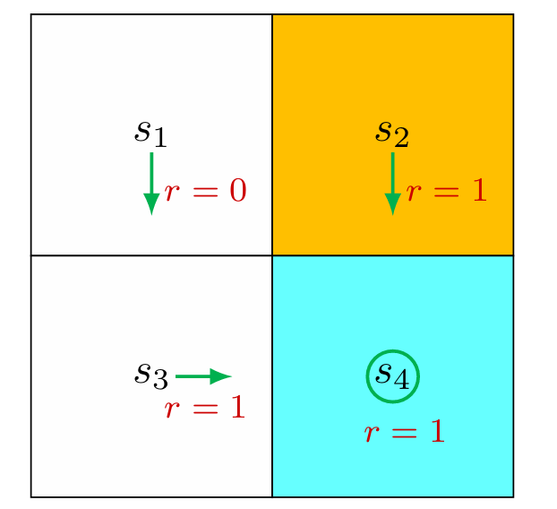
Consider the first example shown in Figure 2.4, where the policy is deterministic. We next write out the Bellman equation and then solve the state values from it.

$$\begin{aligned} & v_\pi\left(s_1\right)=0+\gamma v_\pi\left(s_3\right), \\ & v_\pi\left(s_2\right)=1+\gamma v_\pi\left(s_4\right), \\ & v_\pi\left(s_3\right)=1+\gamma v_\pi\left(s_4\right), \\ & v_\pi\left(s_4\right)=1+\gamma v_\pi\left(s_4\right) . \end{aligned}$$

We can solve the state values from these equations. Since the equations are simple, we can manually solve them. More complicated equations can be solved by the iterative algorithm.

$$\begin{aligned} & v_\pi\left(s_4\right)=\frac{1}{1-\gamma}, \\ & v_\pi\left(s_3\right)=\frac{1}{1-\gamma}, \\ & v_\pi\left(s_2\right)=\frac{1}{1-\gamma}, \\ & v_\pi\left(s_1\right)=\frac{\gamma}{1-\gamma} . \end{aligned}$$

Furthermore, if we set $\gamma=0.9$, then

$$\begin{aligned} & v_\pi\left(s_4\right)=\frac{1}{1-0.9}=10, \\ & v_\pi\left(s_3\right)=\frac{1}{1-0.9}=10, \\ & v_\pi\left(s_2\right)=\frac{1}{1-0.9}=10, \\ & v_\pi\left(s_1\right)=\frac{0.9}{1-0.9}=9 . \end{aligned}$$

2.3.2 For stochastic policy

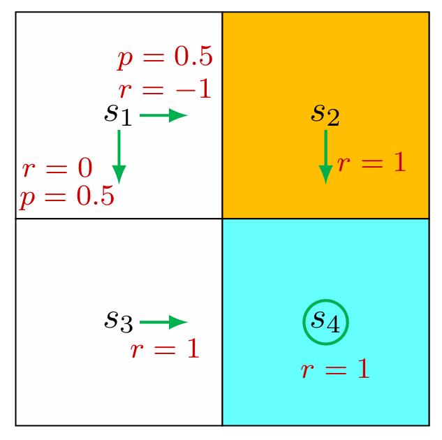
Consider the second example shown in Figure 2.5, where the policy is stochastic. The state transition probability is deterministic, and the reward probability is also deterministic. I,e, the system model is deterministic.

$$v_\pi\left(s_1\right)=0.5\left[0+\gamma v_\pi\left(s_3\right)\right]+0.5\left[-1+\gamma v_\pi\left(s_2\right)\right]$$

Similarly, it can be obtained that

$$\begin{aligned} & v_\pi\left(s_2\right)=1+\gamma v_\pi\left(s_4\right), \\ & v_\pi\left(s_3\right)=1+\gamma v_\pi\left(s_4\right), \\ & v_\pi\left(s_4\right)=1+\gamma v_\pi\left(s_4\right) . \end{aligned}$$

simple, we can solve the state values manually and obtain

$$\begin{aligned} v_\pi\left(s_4\right) & =\frac{1}{1-\gamma}, \\ v_\pi\left(s_3\right) & =\frac{1}{1-\gamma}, \\ v_\pi\left(s_2\right) & =\frac{1}{1-\gamma}, \\ v_\pi\left(s_1\right) & =0.5\left[0+\gamma v_\pi\left(s_3\right)\right]+0.5\left[-1+\gamma v_\pi\left(s_2\right)\right], \\ & =-0.5+\frac{\gamma}{1-\gamma} . \end{aligned}$$

Furthermore, if we set $\gamma=0.9$, then

$$\begin{aligned} & v_\pi\left(s_4\right)=10, \\ & v_\pi\left(s_3\right)=10, \\ & v_\pi\left(s_2\right)=10, \\ & v_\pi\left(s_1\right)=-0.5+9=8.5 . \end{aligned}$$

If we compare the state values of the two policies in the above examples, it can be seen that

$$v_{\pi_1}\left(s_i\right) \geq v_{\pi_2}\left(s_i\right), i= 1,2,3,4$$

which indicates that the policy in Figure 2.4 is better because it has greater state values.
This mathematical conclusion is consistent with the intuition that the rst policy is better because it can avoid entering the forbidden area when the agent starts from s1. As a result, the above two examples demonstrate that state values can be used to evaluate policies.

2.4 Bellman equation: the matrix-vector form

Consider the Bellman equation:

$$\begin{equation} v_\pi(s)=\sum_a \pi(a \mid s)\left[\sum_r p(r \mid s, a) r+\gamma \sum_{s^{\prime}} p\left(s^{\prime} \mid s, a\right) v_\pi\left(s^{\prime}\right)\right] \end{equation}$$

It’s an elementwise form. If we put all the equations together, we have a set of linear equations, which can be concisely written in a matrix-vector form.

Rewrite as

$$v_\pi(s)=r_\pi(s)+\gamma \sum_{s^{\prime}} p_\pi\left(s^{\prime} \mid s\right) v_\pi\left(s^{\prime}\right)$$

where

$$\begin{aligned} & r_\pi(s) \triangleq \sum_a \pi(a \mid s) \sum_r p(r \mid s, a) r, \\ & p_\pi\left(s^{\prime} \mid s\right) \triangleq \sum_a \pi(a \mid s) p\left(s^{\prime} \mid s, a\right) . \end{aligned}$$

Suppose the states could be indexed as $s_i(i=1, \ldots, n)$. For state $s_i$, the Bellman equation is

$$v_\pi\left(s_i\right)=r_\pi\left(s_i\right)+\gamma \sum_{s_j} p_\pi\left(s_j \mid s_i\right) v_\pi\left(s_j\right)$$

Put all these equations for all the states together and rewrite to a matrix-vector form

$$\begin{equation} v_\pi=r_\pi+\gamma P_\pi v_\pi \end{equation}$$

where

$v_\pi=\left[v_\pi\left(s_1\right), \ldots, v_\pi\left(s_n\right)\right]^T \in \mathbb{R}^n$,

$r_\pi=\left[r_\pi\left(s_1\right), \ldots, r_\pi\left(s_n\right)\right]^T \in \mathbb{R}^n$,

$P_\pi \in \mathbb{R}^{n \times n}$, where $\left[P_\pi\right]_{i j}=p_\pi\left(s_j \mid s_i\right)$, is the state transition matrix.

Examples: If there are four states, $v_\pi=r_\pi+\gamma P_\pi v_\pi$ can be written out as

$$\underbrace{\left[\begin{array}{l} v_\pi\left(s_1\right) \\ v_\pi\left(s_2\right) \\ v_\pi\left(s_3\right) \\ v_\pi\left(s_4\right) \end{array}\right]}_{v_\pi}=\underbrace{\left[\begin{array}{l} r_\pi\left(s_1\right) \\ r_\pi\left(s_2\right) \\ r_\pi\left(s_3\right) \\ r_\pi\left(s_4\right) \end{array}\right]}_{r_\pi}+\gamma \underbrace{\left[\begin{array}{llll} p_\pi\left(s_1 \mid s_1\right) & p_\pi\left(s_2 \mid s_1\right) & p_\pi\left(s_3 \mid s_1\right) & p_\pi\left(s_4 \mid s_1\right) \\ p_\pi\left(s_1 \mid s_2\right) & p_\pi\left(s_2 \mid s_2\right) & p_\pi\left(s_3 \mid s_2\right) & p_\pi\left(s_4 \mid s_2\right) \\ p_\pi\left(s_1 \mid s_3\right) & p_\pi\left(s_2 \mid s_3\right) & p_\pi\left(s_3 \mid s_3\right) & p_\pi\left(s_4 \mid s_3\right) \\ p_\pi\left(s_1 \mid s_4\right) & p_\pi\left(s_2 \mid s_4\right) & p_\pi\left(s_3 \mid s_4\right) & p_\pi\left(s_4 \mid s_4\right) \end{array}\right]}_{P_\pi} \underbrace{\left[\begin{array}{l} v_\pi\left(s_1\right) \\ v_\pi\left(s_2\right) \\ v_\pi\left(s_3\right) \\ v_\pi\left(s_4\right) \end{array}\right]}_{v_\pi} .$$

For the above deterministic policy

$$\left[\begin{array}{l} v_\pi\left(s_1\right) \\ v_\pi\left(s_2\right) \\ v_\pi\left(s_3\right) \\ v_\pi\left(s_4\right) \end{array}\right]=\left[\begin{array}{l} 0 \\ 1 \\ 1 \\ 1 \end{array}\right]+\gamma\left[\begin{array}{llll} 0 & 0 & 1 & 0 \\ 0 & 0 & 0 & 1 \\ 0 & 0 & 0 & 1 \\ 0 & 0 & 0 & 1 \end{array}\right]\left[\begin{array}{l} v_\pi\left(s_1\right) \\ v_\pi\left(s_2\right) \\ v_\pi\left(s_3\right) \\ v_\pi\left(s_4\right) \end{array}\right]$$

For the above stochastic policy:

$$\left[\begin{array}{c} v_\pi\left(s_1\right) \\ v_\pi\left(s_2\right) \\ v_\pi\left(s_3\right) \\ v_\pi\left(s_4\right) \end{array}\right]=\left[\begin{array}{c} 0.5(0)+0.5(-1) \\ 1 \\ 1 \\ 1 \end{array}\right]+\gamma\left[\begin{array}{cccc} 0 & 0.5 & 0.5 & 0 \\ 0 & 0 & 0 & 1 \\ 0 & 0 & 0 & 1 \\ 0 & 0 & 0 & 1 \end{array}\right]\left[\begin{array}{l} v_\pi\left(s_1\right) \\ v_\pi\left(s_2\right) \\ v_\pi\left(s_3\right) \\ v_\pi\left(s_4\right) \end{array}\right]$$

2.5 Solving state values from the Bellman equation

Calculating the state values of a given policy is a fundamental problem in reinforcement learning. This problem is often referred to as policy evaluation. In this section, two methods are presented for calculating state values from the Bellman equation.

• The closed-form solution is:

  $$v_\pi=\left(I-\gamma P_\pi\right)^{-1} r_\pi$$

  The drawback of closed-form solution is that it involves a matrix inverse operation, which is computationally expensive. Thus, in practice, we’ll use an iterative algorithm.

• An iterative solution is:

  $$v_{k+1}=r_\pi+\gamma P_\pi v_k \quad k=0,1,2,\dots ,$$

  where $I$ is the identity matrix. We can just randomly select a matrix $v_0$, then calculate $v_1, v_2, \cdots$. This leads to a sequence $\left\{v_0, v_1, v_2, \ldots\right\}$. We can show that

  $$v_k \rightarrow v_\pi=\left(I-\gamma P_\pi\right)^{-1} r_\pi, \quad k \rightarrow \infty$$

Proof: the iterative solution（Contraction mapping theorem）
Define the error as $\delta_k=v_k-v_\pi$. We only need to show $\delta_k \rightarrow 0$. Substituting: $v_{k+1}=\delta_{k+1}+v_\pi$,and $v_k=\delta_k+v_\pi$ into $v_{k+1}=r_\pi+\gamma P_\pi v_k$ gives

$$\delta_{k+1}+v_\pi=r_\pi+\gamma P_\pi\left(\delta_k+v_\pi\right)$$

which can be rewritten as

$$\delta_{k+1}=-v_\pi+r_\pi+\gamma P_\pi \delta_k+\gamma P_\pi v_\pi=\gamma P_\pi \delta_k$$

As a result,

$$\delta_{k+1}=\gamma P_\pi \delta_k=\gamma^2 P_\pi^2 \delta_{k-1}=\cdots=\gamma^{k+1} P_\pi^{k+1} \delta_0$$

Note that $0 \leq P_\pi^k \leq 1$, which means every entry of $P_\pi^k$ is no greater than 1 for any $k=0,1,2, \ldots$. That is because $P_\pi^k =\mathbf{1}$, where $\mathbf{1}=[1, \ldots, 1]^T$. On the other hand, since $\gamma<1$, we know $\gamma^k \rightarrow 0$ and hence $\delta_{k+1} \rightarrow 0$ as $k \rightarrow \infty$.

2.6 Action Value

From state value to action value:

• State value: the average return the agent can get starting from a state.
• Action value: the average return the agent can get starting from a state and taking an action.

Definition of action value (or action value function):

$$\begin{equation} q_\pi(s, a) \triangleq \mathbb{E}\left[G_t \mid S_t=s, A_t=a\right] \end{equation}$$

Note:

1. The $q_\pi(s, a)$ is a function of the state-action pair $(s, a)$.
2. The $q_\pi(s, a)$ depends on $\pi$.

Relation to the state value function

It follows from the properties of conditional expectation that

$$\underbrace{\mathbb{E}\left[G_t \mid S_t=s\right]}_{v_\pi(s)}=\sum_a \underbrace{\mathbb{E}\left[G_t \mid S_t=s, A_t=a\right]}_{q_\pi(s, a)} \pi(a \mid s)$$

Hence,

$$\begin{equation} v_\pi(s)=\sum_a \pi(a \mid s) q_\pi(s, a) \end{equation}$$

Recall the Bellman equation, that the state value is given by

$$v_\pi(s)=\sum_a \pi(a \mid s)[\underbrace{\sum_r p(r \mid s, a) r+\gamma \sum_{s^{\prime}} p\left(s^{\prime} \mid s, a\right) v_\pi\left(s^{\prime}\right)}_{q_\pi(s, a)}]$$

By comparing and , we have the action-value function as

$$\begin{equation} q_\pi(s, a)=\sum_r p(r \mid s, a) r+\gamma \sum_{s^{\prime}} p\left(s^{\prime} \mid s, a\right) v_\pi\left(s^{\prime}\right) \end{equation}$$

equation (5) and equation (6) are the two sides of the same coin:

• equation (5) shows how to obtain state values from action values.
• equation (6) shows how to obtain action values from state values.

Example

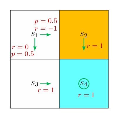
Consider the stochastic policy shown in Figure 2.8.

$$q_\pi\left(s_1, a_2\right)=-1+\gamma v_\pi\left(s_2\right)$$

Note that even if an action would not be selected by a policy, it still has an action value. Therefor, for the other actions:

$$\begin{aligned} & q_\pi\left(s_1, a_1\right)=-1+\gamma v_\pi\left(s_1\right), \\ & q_\pi\left(s_1, a_3\right)=0+\gamma v_\pi\left(s_3\right), \\ & q_\pi\left(s_1, a_4\right)=-1+\gamma v_\pi\left(s_1\right), \\ & q_\pi\left(s_1, a_5\right)=0+\gamma v_\pi\left(s_1\right) . \end{aligned}$$

NOTE:
Although some actions cannot be possibly selected by a given policy, this does not mean that these actions are not good. It is possible that the given policy is not good, so it cannot select the best action. The purpose of reinforcement learning is to find optimal policies. To that end, we must keep exploring all actions to determine better actions for each state.

2.7 Summary

The most important concept introduced in this chapter is the state value. Mathematically, a state value is the expected return that the agent can obtain by starting from a state. The values of different states are related to each other. That is, the value of state $s$ relies on the values of some other states, which may further rely on the value of state $s$ itself. This phenomenon might be the most confusing part of this chapter for beginners. It is related to an important concept called bootstrapping, which involves calculating something from itself. Although bootstrapping may be intuitively confusing, it is clear if we examine the matrix-vector form of the Bellman equation. In particular, the Bellman equation is a set of linear equations that describe the relationships between the values of all states.

Since state values can be used to evaluate whether a policy is good or not, the process of solving the state values of a policy from the Bellman equation is called policy evaluation. As we will see later in this book, policy evaluation is an important step in many reinforcement learning algorithms.

Another important concept, action value, was introduced to describe the value of taking one action at a state. As we will see later in this book, action values play a more direct role than state values when we attempt to find optimal policies. Finally, the Bellman equation is not restricted to the reinforcement learning field. Instead, it widely exists in many elds such as control theories and operation research. In different elds, the Bellman equation may have different expressions. In this book, the Bellman equation is studied under discrete Markov decision processes.

How to calculate action value

• We can first calculate all the state values and then calculate the action values.

• We can also directly calculate the action values with or without models (discussed later).

---

3. Bellman Optimality Equation(BOE)

3.1 Optimal State values and Policy

The state value could be used to evaluate policy : if

$$v_{\pi_1}(s) \geq v_{\pi_2}(s) \quad \text { for all } s \in \mathcal{S}$$

then $\pi_1$ is said to be better than $\pi_2$.

Definition 1(Optimal policy and optimal state value). A policy $\pi^\ast$
is optimal if $v_{\pi^\ast}(s) \geq v_\pi(s)$ for all $s\in S$ and for any other policy $\pi$. The state values $\pi^\ast$ of are the optimal state values.

The definition leads to many questions:

• Does the optimal policy exist?
• Is the optimal policy unique?
• Is the optimal policy stochastic or deterministic?
• How to obtain the optimal policy?

These fundamental questions must be clearly answered to thoroughly understand optimal policies. For example, regarding the existence of optimal policies, if optimal policies do not exist, then we do not need to bother to design algorithms to find them. To answer these questions, we study the Bellman optimality equation.

3.2 Bellman optimality equation (elementwise form)

Bellman optimality equation (BOE) is a tool for analyzing optimal policies and optimal state values. By solving this equation, we can obtain optimal policies and optimal state values.

For every $s \in \mathcal{S}$, the elementwise expression of the BOE is

$$\begin{aligned} v(s) & =\max _{\pi(s) \in \Pi(s)} \sum_{a \in \mathcal{A}} \pi(a \mid s)\left(\sum_{r \in \mathcal{R}} p(r \mid s, a) r+\gamma \sum_{s^{\prime} \in \mathcal{S}} p\left(s^{\prime} \mid s, a\right) v\left(s^{\prime}\right)\right) \\ & =\max _{\pi(s) \in \Pi(s)} \sum_{a \in \mathcal{A}} \pi(a \mid s) q(s, a), \end{aligned}$$

where $v(s), v\left(s^{\prime}\right)$ are unknown variables to be solved and

$$q(s, a) \doteq \sum_{r \in \mathcal{R}} p(r \mid s, a) r+\gamma \sum_{s^{\prime} \in \mathcal{S}} p\left(s^{\prime} \mid s, a\right) v\left(s^{\prime}\right)$$

Here, $\pi(s)$ denotes a policy for state $s$, and $\Pi(s)$ is the set of all possible policies for $s$.

Notes:

$p(r \mid s, a), p\left(s^{\prime} \mid s, a\right)$ are known and $r$,$\gamma$ are designed. this equation has two unknown variables $v(s)$ and $\pi(a \mid s)$. It may be confusing to beginners how to solve two unknown variables from one equation. The reason is this equation satisfy a special quality.(contraction mapping theorem)

3.2.1 Maximize on the right-hand side of BOE

In practice we need to deal with the matrix-vector form since that is what we’re faced with. But since each row in the matrix is actually a vector of the elementwise form, we start with the element form.

In fact, we can turn the problem into “solve the optimal $\pi$ on the right-hand side, next to get the optimal state values “. Let’s look at one example first:

---

Example 1. Consider two unknown variables $x, y \in \mathbb{R}$ that satisfy

$$x=\max _{y \in \mathbb{R}}\left(2 x-1-y^2\right) .$$

The first step is to solve $y$ on the right-hand side of the equation. Regardless of the value of $x$, we always have $\max _y\left(2 x-1-y^2\right)=2 x-1$, where the maximum is achieved when $y=0$. The second step is to solve $x$. When $y=0$, the equation becomes $x=2 x-1$, which leads to $x=1$. Therefore, $y=0$ and $x=1$ are the solutions of the equation.

Example 2. Given $q_1, q_2, q_3 \in \mathbb{R}$, we would like to find the optimal values of $c_1, c_2, c_3$ to maximize

$$\sum_{i=1}^3 c_i q_i=c_1 q_1+c_2 q_2+c_3 q_3,$$

where $c_1+c_2+c_3=1$ and $c_1, c_2, c_3 \geq 0$.
Without loss of generality, suppose that $q_3 \geq q_1, q_2$. Then, the optimal solution is $c_3^\ast=1$ and $c_1^\ast=c_2^\ast=0$. This is because

$$q_3=\left(c_1+c_2+c_3\right) q_3=c_1 q_3+c_2 q_3+c_3 q_3 \geq c_1 q_1+c_2 q_2+c_3 q_3$$

for any $c_1, c_2, c_3$.

---

Inspired by the above example, since $\sum_a(\pi(a \mid s))= 1$, the (elementwise) BOE can be written as

$$v(s)=\max _{\pi(s) \in \Pi(s)} \sum_{a \in \mathcal{A}} \pi(a \mid s) q(s, a)\quad =\max _{a \in \mathcal{A}(s)} q(s, a) , s \in \mathcal{S}.$$

where the optimality is achieved when

$$\pi(a \mid s)= \begin{cases}1 & a=a^* \\ 0 & a \neq a^*\end{cases}$$

where $a^*=\arg \max _a q(s, a)$(arg is get the variant value).

In summary, the optimal policy $\pi(s)$ is the one that selects the action that has the greatest value of $q(s,a)$.

Now that we know the solution of BOE is to maximize the right-hand side, - just select the greatest action value $q(s,a)$. But we don’t know action value or state value at this time, next , we need study how to obtain state value from the contraction mapping theorem on the matrix-vector form.

3.2.2 Matrix-vector form of the BOE

To leverage the contraction mapping theorem, we’ll express the matrix-vector form as

$$\begin{equation} v =\max _{\pi \in \mathcal{\pi}}\left(r_\pi+\gamma P_\pi v\right) . \end{equation}$$

where $v \in \mathbb{R}^{|\mathcal{S}|}$ and $\max _\pi$ is performed in an elementwise manner. The structures of $r_\pi$ and $P_\pi$ are the same as those in the matrix-vector form of the normal Bellman equation:

$$\left[r_\pi\right]_s \doteq \sum_{a \in \mathcal{A}} \pi(a \mid s) \sum_{r \in \mathcal{R}} p(r \mid s, a) r, \quad\left[P_\pi\right]_{s, s^{\prime}}=p\left(s^{\prime} \mid s\right) \doteq \sum_{a \in \mathcal{A}} \pi(a \mid s) p\left(s^{\prime} \mid s, a\right) .$$

Since the optimal value of $\pi$ is determined by $v$, the right-hand side of BOE (matrix-vector form) is a function of $v$, denoted as

$$\begin{equation} f(v) \triangleq \max _{\pi}\left(r_\pi+\gamma P_\pi v\right) . \end{equation}$$

Then, the BOE can be expressed in a concise form as

$$v=f(v)$$

Every row $[f(v)]_s$ is the elementwise form of $s$.

3.2.3 Contraction mapping theorem

Now that the matrix-vector form is expressed as a nonlinear equation $v = f(v)$, we next introduce the contraction mapping theorem to analyze it. The contraction mapping theorem is a powerful tool for analyzing general nonlinear equations.

Concepts: Fixed point and Contraction mapping

Fixed point: $x^\ast \in X$ is a fixed point of $f: X \rightarrow X$ if

$$f(x^*)=x^*$$

Contraction mapping (or contractive function): $f$ is a contraction mapping if

$$\left\|f\left(x_1\right)-f\left(x_2\right)\right\| \leq \gamma\left\|x_1-x_2\right\|$$

where $\gamma \in(0,1)$. $|\cdot|$ denotes a vector or matrix norm.

Example1
Given $x=f(x)=A x$, where $x \in \mathbb{R}^n, A \in \mathbb{R}^{n \times n}$ and $|A| \leq \gamma<1$.
It is easy to verify that $x=0$ is a fixed point since $0=A 0$. To see the contraction property,

$$\left\|A x_1-A x_2\right\|=\left\|A\left(x_1-x_2\right)\right\| \leq\|A\|\left\|x_1-x_2\right\| \leq \gamma\left\|x_1-x_2\right\| .$$

Therefore, $f(x)=A x$ is a contraction mapping.

Theorem: Contraction Mapping Theorem
For any equation that has the form of $x=f(x)$,where $x$ and $f(x)$ are real vectors if $f$ is a contraction mapping, then the following peoperties hold.

• Existence: there exists a fixed point $x^\ast$ satisfying $f\left(x^\ast\right)=x^\ast$.
• Uniqueness: The fixed point $x^*$ is unique.
• Algorithm: Consider a sequence $\left\{x_k\right\}$ where $x_{k+1}=f\left(x_k\right)$, then $x_k \rightarrow x^*$( fixed point) as $k \rightarrow \infty$ for any initial guess $x_0$. Moreover, the convergence rate is exponentially fast.

-> See the proof

3.3 Contraction property of the BOE

Theorem (Contraction Property):

$f(v)$ is a contraction mapping satisfying

$$\left\|f\left(v_1\right)-f\left(v_2\right)\right\|_{\infty} \leq \gamma\left\|v_1-v_2\right\|_{\infty}$$

where $\gamma \in(0,1)$ is the discount rate, and $|\cdot|_{\infty}$ is the maximum norm, which is the maximum absolute value of the elements of a vector.

-> See the proof

3.4 Solution of the BOE

Due to the contraction property of BOE, the matrix-vector form can be solved by computing following equation iteratively

$$\begin{equation} v_{k+1}=f\left(v_k\right)=\max _\pi\left(r_\pi+\gamma P_\pi v_k\right) . \end{equation}$$

At every iteration, for each state, what we face is actually the elementwise form:

$$\begin{aligned} v_{k+1}(s) & =\max _\pi \sum_a \pi(a \mid s)\left(\sum_r p(r \mid s, a) r+\gamma \sum_{s^{\prime}} p\left(s^{\prime} \mid s, a\right) v_k\left(s^{\prime}\right)\right) \\ & =\max _\pi \sum_a \pi(a \mid s) q_k(s, a) \\ & =\max _a q_k(s, a) . \end{aligned}$$

Procedure summary (value iteration algorithm):
For every $s$, estimate(randomly select) current state value as $v_k(s)$
For any $a \in \mathcal{A}(s)$, calculate

$$q_k(s, a)=\sum_r p(r \mid s, a) r+\gamma \sum_{s^{\prime}} p\left(s^{\prime} \mid s, a\right) v_k\left(s^{\prime}\right)$$

Calculate the greedy policy $\pi_{k+1}$ for every $s$ as

$$\pi_{k+1}(a \mid s)=\left\{\begin{array}{cc} 1 & a=a_k^*(s) \\ 0 & a \neq a_k^*(s) \end{array}\right.$$

where $a_k^*(s)=\arg \max _a q_k(s, a)$.
Calculate $v_{k+1}(s)=\max _a q_k(s, a)$

3.5 BOE: Optimality

Suppose $v^*$ is the solution to the Bellman optimality equation. It satisfies

$$v^*=\max _\pi\left(r_\pi+\gamma P_\pi v^*\right)$$

Suppose

$$\pi^*=\arg \max _\pi\left(r_\pi+\gamma P_\pi v^*\right)$$

Then

$$v^*=r_{\pi^*}+\gamma P_{\pi^*} v^*$$

Therefore, $ \pi^\ast $ is a policy and $ v^\ast=v_{\pi^\ast} $,and the BOE is a special Bellman equation whose corresponding policy is $ \pi^\ast $.

3.6 What does $\pi^\ast$ look like?

For any $s \in \mathcal{S}$, the deterministic greedy policy

$$\pi^*(a \mid s)= \begin{cases}1 & a=a^*(s) \\ 0 & a \neq a^*(s)\end{cases}$$

is an optimal policy solving the BOE. Here,

$$a^*(s)=\arg \max _a q^*(a, s)$$

where $ q^\ast(s, a):=\sum_r p(r \mid s, a) r+\gamma \sum_{s^{\prime}} p\left(s^{\prime} \mid s, a\right) v^\ast\left(s^{\prime}\right) $.

Proof: Due to

$$\pi^*(s)=\arg \max _{\pi \in \Pi} \sum_{a \in \mathcal{A}} \pi(a \mid s) \underbrace{\left(\sum_{r \in \mathcal{R}} p(r \mid s, a) r+\gamma \sum_{s^{\prime} \in \mathcal{S}} p\left(s^{\prime} \mid s, a\right) v^*\left(s^{\prime}\right)\right)}_{q^*(s, a)}, \quad s \in \mathcal{S} .$$

It is clear that $ \sum_{a \in \mathcal{A}} \pi(a \mid s) q^\ast(s, a) $ is maximized if $ \pi(s) $ selects the action with the greatest $ q^\ast(s, a) $.

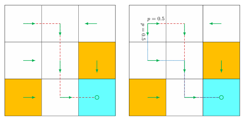
Uniqueness of optimal policies: Although the value of $ v^\ast $ is unique, the optimal policy that corresponds to $ v^\ast $ may not be unique. This can be easily verified by counterexamples. For example, the two policies shown in below Figure are both optimal.
Stochasticity of optimal policies: An optimal policy can be either stochastic or deterministic, as demonstrated in below Figure. However, it is certain that there always exists a deterministic optimal policy.

3.7 Factors that influence optimal policies

$$\pi^*(s)=\arg \max _{\pi \in \Pi(s)} \sum_{a \in \mathcal{A}} \pi(a \mid s) \left(\sum_{r \in \mathcal{R}} p(r \mid s, a) r+\gamma \sum_{s^{\prime} \in \mathcal{S}} p\left(s^{\prime} \mid s, a\right) v^*\left(s^{\prime}\right)\right), \quad s \in \mathcal{S} .$$

The optimal state value and optimal policy are determined by the following parameters: 1) the immediate reward $r$, 2) the discount rate $\gamma$, and 3) the system model
$p(s^{\prime} \mid s,a), p(r \mid s,a)$. While the system model is fixed, we next discuss how the optimal policy varies when we change the values of $r$ and $\gamma$.

Impact of the discount rate and the reward values

• $\gamma$ from 0 to 1 , each state from extremely short-sighted to far-sighted

• if a state must travel along a longer trajectory to reach the target, its state value is smaller due to the discount rate.Therefore, although the immediate reward of every step does not encourage the agent to approach the target as quickly as possible, the discount rate does encourage it to do so.

• If we want to strictly prohibit the agent from entering any forbidden area, we can increase the punishment received for doing so.

Theorem (Optimal policy invariance)(Linear variation):

Consider a Markov decision process with $v^\ast \in \mathbb{R}^{|\mathcal{S}|}$ as the optimal state value satisfying $v^\ast=\max _{\pi \in \Pi}\left(r_\pi+\gamma P_\pi v^\ast\right)$. If every reward $r \in \mathcal{R}$ is changed by an affine transformation to $\alpha r+\beta$, where $\alpha, \beta \in \mathbb{R}$ and $\alpha>0$, then the corresponding optimal state value $v^{\prime}$ is also an affine transformation of $v^\ast$ :

$$v^{\prime}=\alpha v^*+\frac{\beta}{1-\gamma} \mathbf{1}$$

where $\gamma \in(0,1)$ is the discount rate and $\mathbf{1}=[1, \ldots, 1]^T$.

Consequently, the optimal policy derived from $v^{\prime}$ is invariant to the affine transformation of the reward values.

3.8 Summary

The core concepts in this chapter include optimal policies and optimal state values. In particular, a policy is optimal if its state values are greater than or equal to those of any other policy. The state values of an optimal policy are the optimal state values. The BOE is the core tool for analyzing optimal policies and optimal state values. This equation is a nonlinear equation with a nice contraction property. We can apply the contraction mapping theorem to analyze this equation. It was shown that the solutions of the BOE correspond to the optimal state value and optimal policy. This is the reason why we need to study the BOE.

Q: What is the definition of optimal policies?
A: A policy is optimal if its corresponding state values are greater than or equal to any other policy. It should be noted that this specific definition of optimality is valid only for tabular reinforcement learning algorithms. When the values or policies are approximated by functions, different metrics must be used to define optimal policies. This will become clearer in Chapters 8 and 9.

Q: Are optimal policies stochastic or deterministic?
A: An optimal policy can be either deterministic or stochastic. A nice fact is that there always exist deterministic greedy optimal policies.

Q: If we increase all the rewards by the same amount, will the optimal state value change? Will the optimal policy change?
A: Increasing all the rewards by the same amount is an affine transformation of the rewards, which would not affect the optimal policies. However, the optimal state value would increase, as shown in (Optimal policy invariance).