[toc]
Sources:
6 Stochastic Approximation
We use the present chapter to fill this knowledge gap by introducing the basics of stochastic approximation. Although this chapter does not introduce any specific reinforcement learning algorithms, it lays the necessary foundations for studying subsequent chapters. We will see in Chapter 7 that the temporal-difference algorithms can be viewed as special stochastic approximation algorithms. The well-known stochastic gradient descent (SGD) algorithms widely used in machine learning are also introduced in the present chapter.
6.1 Mean estimation
The basic idea of Monte Carlo estimation is:
as $n$ increases, the approximation becomes increasingly accurate. When $n \rightarrow \infty$, we have $\bar{x} \rightarrow \mathbb{E}[X]$.
We next show that two methods can be used to calculate $\bar{x}$ . The first non-incremental method collects all the samples first and then calculates the average. The drawback of such a method is that, if the number of samples is large, we may have to wait for a long time until all of the samples are collected.
The second method can avoid this drawback because it calculates the average in an incremental manner Specifically, suppose that:
Therefore, we obtain the following incremental algorithm:
The advantage of the incremental algorithm is that the average can be immediately calculated every time we receive a sample. This average can be used to approximate $\bar{x}$ and hence $\mathbb{E}[X]$. Notably, the approximation may not be accurate at the beginning due to insufficient samples. However, it is better than nothing.
Furthermore, consider an algorithm with a more general expression:
It is the same as the incremental algorithm except that the coefficient $1/k$ is replaced by $a_k > 0$ However, we will show in the next section that, if $k$ satisfies some mild conditions, $w_k \rightarrow \mathbb{E}[X]$ as $k \rightarrow \infty$. In Chapter 7, we will see that temporal-difference algorithms have similar (but more complex) expressions.
6.2 Robbins-Monro (RM) algorithm
Robbins-Monro (RM) algorithm: solve $g(w)=0$ using $\left\{\tilde{g}\left(w_k, \eta_k\right)\right\}$
Stochastic approximation refers to a broad class of stochastic iterative algorithms solving root finding or optimization problems. Compared to many other root-finding algorithms such as gradient-based methods, Stochastic approximation is powerful in the sense that it does not require the expression of the objective function nor its derivative.
Robbins-Monro (RM) algorithm is a pioneering work in the field of stochastic approximation. The famous stochastic gradient descent (SGD) algorithm is a special form of the RM algorithm.
6.2.1 Problem statement
Problem statement: Suppose we would like to find the root of the equation
where $w \in \mathbb{R}$ is the variable to be solved and $g: \mathbb{R} \rightarrow \mathbb{R}$ is a function. Many problems can be formulated as root- finding problems. For example, if $J(w)$ is an objective function to be optimized, this optimization problem can be converted to solving $g(w) = \nabla_w J(w) = 0$.
If the expression of $g$ or its derivative is known, there are many numerical algorithms that can solve this problem.However, the problem we are facing is that the expression of the function g is unknown. For example, the function may be represented by an artificial neural network whose structure and parameters are unknown. Moreover, we can only obtain a noisy observation of $g(w)$:
where $\eta \in \mathbb{R}$ is the observation error, which may or may not be Gaussian. In summary, it is a black-box system where only the input $w$ and the noisy output $\tilde{g}(w, \eta)$ are known. Our aim is to solve $g(w)=0$ using $w$ and $\tilde{g}$.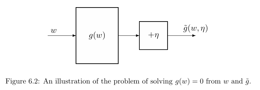
The Robbins-Monro (RM) algorithm can solve $g(w)=0$ is
where $w_k$ is the $k$ th estimate of the root, $\tilde{g}\left(w_k, \eta_k\right)=g\left(w_k\right)+\eta_k$ is the $k$ th noisy observation $a_k$ is a positive coefficient. As can been seen, RM algorithm only requires the input ($\left\{w_k\right\}$) and output data ($\left\{\tilde{g}\left(w_k, \eta_k\right)\right\}$). It does not need to know the expression of $g(w)$. Next we introduce an example to illustrate RM algorithm.
6.2.2 An illustrative example
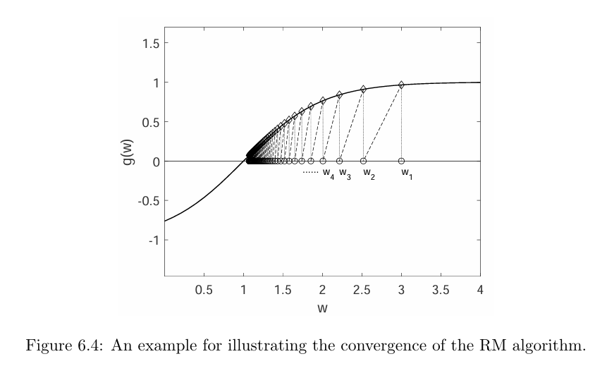
Consider the example shown in Figure. In this example, $g(w)=\tanh (w-1)$, the true root of $g(w)=0$ is $w^\ast=1$. Parameters: $w_1=3, a_k=1 / k, \eta_k \equiv 0$ (no noise for the sake of simplicity) The RM algorithm in this case is $\textcolor{blue} {w_{k+1}=w_k-a_k g\left(w_k\right)} $ since $\tilde{g}\left(w_k, \eta_k\right)=g\left(w_k\right)$ when $\eta_k=0$. The resulting $\left\{w_k\right\}$ generated by the RM algorithm is shown in Figure . It can be seen that $w_k$ converges to the true root $w^\ast=1$.
This simple example can illustrate why the RM algorithm converges.
- When $w_k>w^\ast$, we have $g\left(w_k\right)>0$. Then, $w_{k+1}=w_k-a_k g\left(w_k\right)<w_k$. If $a_k g\left(w_k\right)$ is sufficiently small, we have $w^\ast<w_{k+1}<w_k$. As a result, $w_{k+1}$ is closer to $w^\ast$ than $w_k$.
- When $w_k
In either case,$w_{k+1}$ is closer to $w^\ast$ than $w_k$. Therefore, it is intuitive that $w_k$ converges to $w^\ast$.
6.2.3 RM algorithm’s proof
Robbins-Monro theorem: In the Robbins-Monro algorithm $\textcolor{red} {w_{k+1}=w_k-a_k \tilde{g}\left(w_k, \eta_k\right) ,k=1,2,3,\dots}$, if:
(a) $0<c_1 \leq \nabla_w g(w) \leq c_2$ for all $w$;
(b) $\sum_{k=1}^{\infty} a_k=\infty$ and $\sum_{k=1}^{\infty} a_k^2<\infty$;
(c) $\mathbb{E}\left[\eta_k \mid \mathcal{H}_k\right]=0$ and $\mathbb{E}\left[\eta_k^2 \mid \mathcal{H}_k\right]<\infty$;
where $\mathcal{H}_k=\left\{w_k, w_{k-1}, \ldots\right\}$, then $w_k$ almost surely converges to the root $w^\ast$ satisfying $g\left(w^\ast\right)=0$.
The three conditions in previous are explained as follows.
Condition (a)
$0<c_1 \leq \nabla_w g(w)$ indicates that $g(w)$ is a monotonically increasing function. This condition ensures that the root of $g(w)=0$ exists and is unique. If $g(w)$ is monotonically decreasing, we can simply treat $-g(w)$ as a new function that is monotonically increasing.
As an application, we can formulate an optimization problem in which the objective function is $J(w)$ as a root- finding problem: $g(w) = \nabla_wJ(w) = 0$. In this case, the condition that $g(w)$ is monotonically increasing indicates that $J(w)$ is convex, which is a commonly adopted assumption in optimization problems.
The inequality $\nabla_w g(w) \leq c_2$ indicates that the gradient of $g(w)$ is bounded from above. For example, $g(w)=\tanh (w-1)$ satisfies this condition, but $g(w)=w^3-5$ does not.
Condition (b)
The second condition about $\left\{a_k\right\}$ is interesting. We often see conditions like this in reinforcement learning algorithms.
In particular, the condition $\sum_{k=1}^{\infty} a_k^2<\infty$ means that $\lim _{n \rightarrow \infty} \sum_{k=1}^n a_k^2$ is bounded from above. It requires that $a_k$ converges to zero as $k \rightarrow \infty$.
The condition $\sum_{k=1}^{\infty} a_k=\infty$ means that $\lim _{n \rightarrow \infty} \sum_{k=1}^n a_k$ is infinitely large. It requires that $a_k$ should not converge to zero too fast. These conditions have interesting properties, which will be analyzed in detail shortly.
Condition (c)
The condition is mild. It does not require the observation error $\eta_k$ to be Gaussian. An important special case is that $\left\{\eta_k\right\}$ is an i.i.d. stochastic sequence satisfying $\mathbb{E}\left[\eta_k\right]=0$ and $\mathbb{E}\left[\eta_k^2\right]<\infty$. In this case, the third condition is valid because $\eta_k$ is independent of $\mathcal{H}_k$ and hence we have $\mathbb{E}\left[\eta_k \mid \mathcal{H}_k\right]=\mathbb{E}\left[\eta_k\right]=0$ and $\mathbb{E}\left[\eta_k^2 \mid \mathcal{H}_k\right]=\mathbb{E}\left[\eta_k^2\right]$.
Why is the second condition important for the convergence of the RM algorithm?
This question can naturally be answered when we present a rigorous proof of the above theorem later. Here, we would like to provide some insightful intuition.
First, $\sum_{k=1}^{\infty} a_k^2<\infty$ indicates that $a_k \rightarrow 0$ as $k \rightarrow \infty$. Why is this condition important? Suppose that the observation $\tilde{g}\left(w_k, \eta_k\right)$ is always bounded. Since
if $a_k \rightarrow 0$, then $a_k \tilde{g}\left(w_k, \eta_k\right) \rightarrow 0$ and hence $w_{k+1}-w_k \rightarrow 0$, indicating that $w_{k+1}$ and $w_k$ approach each other when $k \rightarrow \infty$.Otherwise, if $a_k$ does not converge, then $w_k$ may still fluctuate when $k \rightarrow \infty$.
Second, $\sum_{k=1}^{\infty} a_k=\infty$ indicates that $a_k$ should not converge to zero too fast. Why is this condition important?
Summarizing both sides of the equations of $ w_2-w_1 = -a_1 \tilde{g}\left(w_1, \eta_1\right), w_3-w_2=-a_2 \tilde{g}\left(w_2, \eta_2\right), w_4-w_3=-a_3 \tilde{g}\left(w_3, \eta_3\right), \ldots $ gives
If $\sum_{k=1}^{\infty} a_k<\infty$, then $\left|\sum_{k=1}^{\infty} a_k \tilde{g}\left(w_k, \eta_k\right)\right|$ is also bounded. But we will show that this can not guarantee the convergence. Let $b$ denote the finite upper bound such that
If the initial guess $w_1$ is selected far away from $w^\ast$ so that $\left|w_1-w^\ast\right|>b$, then it is impossible to have $w_{\infty}=w^\ast$. This suggests that the RM algorithm cannot find the true solution $w^\ast$ in this case. Therefore, the condition $\sum_{k=1}^{\infty} a_k=\infty$ is necessary to ensure convergency given an arbitrary initial guess.
An example of $a_k$
What kinds of sequences satisfy $\sum_{k=1}^{\infty} a_k=\infty$ and $\sum_{k=1}^{\infty} a_k^2<\infty$ ?
One typical sequence is
On the one hand, it holds that
where $\kappa \approx 0.577$ is called the Euler-Mascheroni constant (or Euler’s constant) . Since $\ln n \rightarrow \infty$ as $n \rightarrow \infty$, we have
In fact, $H_n=\sum_{k=1}^n \frac{1}{k}$ is called the harmonic number in number theory [29]. On the other hand, it holds that
Finding the value of $\sum_{k=1}^{\infty} \frac{1}{k^2}$ is known as the Basel problem [30].
In summary, the sequence $\left\{a_k=1 / k\right\}$ satisfies the second condition in Theorem 6.1. Notably, a slight modification, such as $a_k=1 /(k+1)$ or $a_k=c_k / k$ where $c_k$ is bounded, also preserves this condition.
Note:
In the RM algorithm, $a_k$ is often selected as a sufficiently small constant in many applications. Although the second condition is not satisfied anymore in this case because $\sum_{k=1}^{\infty} a_k^2=\infty$ rather than $\sum_{k=1}^{\infty} a_k^2<\infty$, the algorithm can still converge in a certain sense.
6.2.4 Mean estimation is a special example of RM algorithm
In particular, define a function as
The original problem is to obtain the value of $\mathbb{E}[X]$. This problem is formulated as a root- finding problem to solve $g(w) = 0$. Given a value of $w$, the noisy observation that we can obtain is $\tilde{g} = w -x$, where $x$ is a sample of $X$. Note that $\tilde{g}$ can be written as
The RM algorithm for solving this problem is
So, solving $\mathbb{E}(X)$ by mean estimation can be convert to solving a RM algorithm with $g(w) = w-\mathbb{E}(x)$ and $a_k=\frac{1}{k}$.
6.3 Stochastic gradient descent
Stochastic Gradient Descent (SGD) algorithm: minimize $J(w)=\mathbb{E}[f(w, X)]$ using $\left\{\nabla_w f\left(w_k, x_k\right)\right\}$
The iterative mean estimation algorithm is a special form of the Stochastic Gradient Descent (SGD) algorithm, and the SGD algorithm is a special form of the RM algorithm. (IME → SGD → RM)
Consider the following optimization problem:
where $w$ is the parameter to be optimized. $X$ is a random variable. The expectation is with respect to $X$. $w$ and $X$ can be either scalars or vectors. The function $f(\cdot)$ is a scalar.
The gradient descent algorithm (GD)
we must know the probability distribution of $X$, if you want use this algorithm.
The batch gradient descent algorithm (BGD)
We can use Monte Carlo estimation to compute the estimate $\mathbb{E}\left[\nabla_w f\left(w_k, X\right)\right]$.
One problem of the BGD algorithm is that it requires all the samples in each iterationfor each $w_k$.
The stochastic gradient descent algorithm (SGD)
where $x_k$ is the sample collected at time step $k$. It relies on stochastic samples ${x_k}$
Compared to the gradient descent algorithm: Replace the true gradient $\mathbb{E}\left[\nabla_w f\left(w_k, X\right)\right]$ by the stochastic gradient $\nabla_w f\left(w_k, x_k\right)$.
Compared to the batch gradient descent method: let $n=1$.
From GD to SGD: The stochastic gradient $\nabla_w f\left(w_k, x_k\right)$ can be viewed as a noisy measurement of the true gradient $\mathbb{E}\left[\nabla_w f(w, X)\right]$:
Therefore, the perturbation term $\eta_{k}$ has a zero mean, which intuitively suggests that it may not jeopardize the convergence property.
6.3.1 Mean estimation is a special example of SGD
we formulate the mean estimation problem as an optimization problem:
where $ f(w, X)=|w-X|^2 / 2 \quad \nabla_w f(w, X)=w-X $ . It can be verified that the optimal solution is by solving $\textcolor{green} {\nabla_w J(w)=0}$. Therefore, this optimization problem is equivalent to the iterative mean estimation problem.
The SGD algorithm for solving the above problem is
We can therefore see that the iterative mean estimation algorithm is a special form of the SGD algorithm for solving the mean estimation problem.
6.3.2 SGD is a special example of RM algorithm (Convergence analysis)
We next show that SGD is a special RM algorithm, Then, the convergence naturally follows.
The aim of SGD is to minimize
This problem can be converted to a root-finding problem:
Let
Then, the aim of SGD is to find the root of $g(w)=0$.
As in RM algorithm, we don’t know $g(w)$. Knowing it needs GD (gradient descent), not SGD.
What we can measure is
Then, the RM algorithm for solving $g(w)=0$ is
It is exactly the SGD algorithm. Therefore, SGD is a special RM algorithm.Since SGD is a special RM algorithm, its convergence naturally follows.
Theorem (Convergence of SGD): In the SGD algorithm, if
$0<c_1 \leq \nabla_w^2 f(w, X) \leq c_2$;
$\sum_{k=1}^{\infty} a_k=\infty$ and $\sum_{k=1}^{\infty} a_k^2<\infty$;
$\left\{x_k\right\}_{k=1}^{\infty}$ is iid;
then $w_k$ converges to the root of $ \mathbb{E}[\nabla_wf(w, X)]=0$ with probability 1.
6.3.3 Convergence pattern
Since the stochastic gradient is random and hence the approximation is inaccurate, whether the convergence of SGD is slow or random? To answer this question, we consider the relative error between the stochastic and batch gradients:
The relative error between the stochastic and true gradients is
For the sake of simplicity, we consider the case where $w$ and $\nabla_w f(w, x)$ are both scalars. Since $w^\ast$ is the optimal solution, it holds that $\mathbb{E}\left[\nabla_w f\left(w^\ast, X\right)\right]=0$. Then, the relative error can be rewritten as
where the last equality is due to the mean value theorem and $\tilde{w}_k \in\left[w_k, w^\ast\right]$. Suppose that $f$ is strictly convex such that $\nabla_w^2 f \geq c>0$ for all $w, X$. Then, the denominator becomes
Substituting the above inequality into the above equation yields
The above inequality suggests an interesting convergence pattern of SGD: the relative error $\delta_k$ is inversely proportional to $\left|w_k-w^\ast\right|$. As a result, when $\left|w_k-w^\ast\right|$ is large, $\delta_k$ is small. In this case, the SGD algorithm behaves like the gradient descent algorithm and hence $w_k$ quickly converges to $w^\ast$. When $w_k$ is close to $w^\ast$, the relative error $\delta_k$ may be large, and the convergence exhibits more randomness.
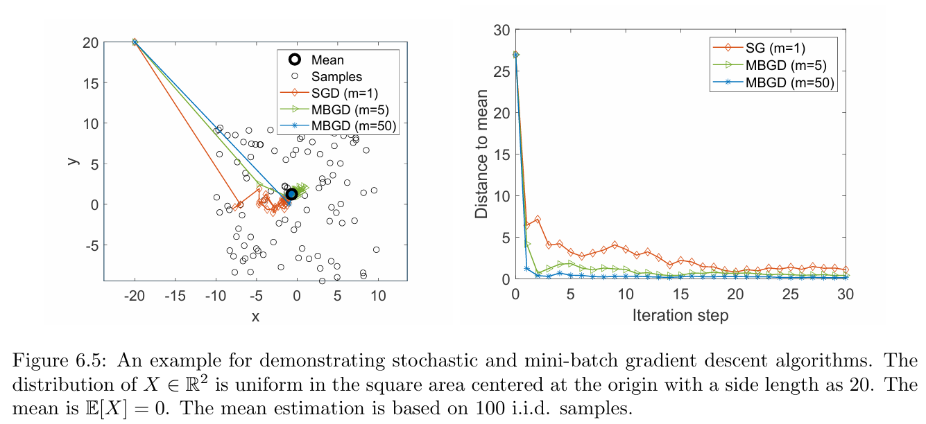
The simulation results are shown in Figure. Here, $X\in \mathbb{R^2}$ represents a random position in the plane. Its distribution is uniform in the square area centered at the origin and $\mathbb{E}[X] = 0$. The mean estimation is based on 100 i.i.d. samples. Although the initial guess of the mean is far away from the true value, it can be seen that the SGD estimate quickly approaches the neighborhood of the origin. When the estimate is close to the origin, the convergence process exhibits certain randomness.
6.3.4 BGD, SGD, and mini-batch GD
| algorithms | sample used in every iteration | randomness | flexible and efficient |
|---|---|---|---|
| SGD | a single sample ($1$) | maximum | maximum |
| MBGD | a few more samples ($1<=m<=n$) | median | median |
| BGD | all samples ($n$) | minimum | minimum |
notes
If $m=n$, MBGD does NOT become BGD strictly speaking, because MBGD uses randomly fetched $n$ samples whereas BGD uses all $n$ numbers. In particular, MBGD may use a value in $\left\{x_i\right\}_{i=1}^n$ multiple times whereas BGD uses each number once.
Suppose we would like to minimize $J(w)=\mathbb{E}[f(w, X)]$, given a set of random samples $\left\{x_i\right\}_{i=1}^n$ of $X$. The BGD, SGD, MBGD algorithms solving this problem are, respectively,
where $n$ is the size of the dataset, $m \leq n$.
In the BGD algorithm, all the samples are used in every iteration. When $n$ is large, $(1 / n) \sum_{i=1}^n \nabla_w f\left(w_k, x_i\right)$ is close to the true gradient $\mathbb{E}\left[\nabla_w f\left(w_k, X\right)\right]$.
In the MBGD algorithm, $\mathcal{I}_k$ is a subset of $\{1, \ldots, n\}$ with the size as $\left|\mathcal{I}_k\right|=m$. The set $\mathcal{I}_k$ is obtained by $m$ times i.d.d. samplings.
In the SGD algorithm, $x_k$ is randomly sampled from $\left\{x_i\right\}_{i=1}^n$ at time $k$.
A good example
Given some numbers $\left\{x_i\right\}_{i=1}^n$, our aim is to calculate the mean $\bar{x}=\sum_{i=1}^n x_i / n$. This problem can be equivalently stated as the following optimization problem:
The three algorithms for solving this problem are, respectively,
where $\bar{x}_k^{(m)}=\sum_{j \in \mathcal{I}_k} x_j / m$. Furthermore, if $\alpha_k=1 / k$, the above equation can be solved as
The estimate of BGD at each step is exactly the optimal solution $w^\ast=\bar{x}$.
The estimate of MBGD converges the mean faster than SGD because $\bar{x}_k^{(m)}$ is already an average.
the convergence rate of SGD is still fast, especially when $w_k$ is far from $w^\ast$.
6.4 Summary
This chapter introduced the preliminaries of stochastic approximation such as the RM and SGD algorithms. Compared to many other root-finding algorithms, the RM algorithm does not require the expression of the objective function or its derivative. It has been shown that the SGD algorithm is a special RM algorithm. Moreover, an important problem frequently discussed throughout this chapter is mean estimation. The mean estimation algorithm is a special SGD algorithm. We will see in Chapter 7 that temporal-difference learning algorithms have similar expressions. Finally, the name “stochastic approximation” was first used by Robbins and Monro in 1951 1. More information about stochastic approximation can be found in 2.
1:H. Robbins and S. Monro, A stochastic approximation method, The Annals of
Mathematical Statistics, pp. 400407, 1951.
2. H.-F. Chen, Stochastic approximation and its applications, vol. 64. Springer Science & Business Media, 2006 ↩
7 Temporal-Difference Methods
Temporal-difference (TD) learning is one of the most well-known methods in reinforcement learning (RL).TD learning often refers to a broad class of reinforcement learning algorithms(Sarsa\ Expectded Sarsa\ n-step Sarsa\Q-learning eta).
Monte Carlo (MC) learning and TD learning are the model-free methods. but TD learning has some advantages due to its incremental form.
TD learning algorithms can be viewed as special stochastic algorithms for solving the Bellman or Bellman optimality equations.
7.1 TD learning of state values
7.1.1 Algorithm description
TD algorithm can estimate the state values of a given policy using the following equations:
Suppose that we have some experience samples $(s_0, r_1, s_1,\dots, s_t, r_{t+1}, s_{t+1},\dots)$ generated following .
where $t = 0,1,2,\dots$ denotes the time step. Here, $v_t(s_t)$ is the estimate of $v_\pi(s_t)$ at time $t$; $\alpha_t(s_t)$ is the learning rate for $s_t$ at time $t$. Equation (7) is often omitted for simplicity, but it should be kept in mind because the algorithm would be mathematically incomplete without this equation.
TD learning algorithm can be viewed as a special stochastic approximation
algorithm(i.e. Robbins-Monro algorithm) for solving the Bellman equation.
It is another expression of the Bellman equation which sometimes called the Bellman expectation equation.
Derivation of the TD algorithm
our goal is to solve the $g(v_{\pi}(s_t))=0$ to obtain $v_{\pi}(s_t)$ using the RM algorithm. $r_{t+1}$ and $s_{t+1}$ are the samples of $R_{t+1}$ and $S_{t+1}$,the noisy observation of $g(v_{\pi}(s_t))$ that we can obtain is
Therefore, the Robbins-Monro algorithm (Section 6.2) for solving $g(v_{\pi}(s_t)) = 0$ is
$v_t(s)$ converges almost surely to $v_{\pi}(s)$ as $t \to \infty$ for all $s \in S$
7.1.2 Property analysis (TD target and TD error)
TD algorithm can be described as
TD target : $\tilde{v}_t=r_{t+1}+\gamma v_{t}(s_{t+1})$
Key:The current estimated state value ($\tilde{v}_t$ or $\tilde{v}_t(s_t)$) is obtained by using the next state value $v_t(s_{t+1})$ in time step $t+1$.
TD error :$\delta_t=v_{t}(s_t)-\tilde{v}_t=v_{t}(s_t)-(r_{t+1}+\gamma v_{t}(s_{t+1}))$
Key:the error of the current state value $v_t(s_t)$ with the estimated state value ($\tilde{v}_t$ or $\tilde{v}_t(s_t)$) in time step $t$.
the TD error can be interpreted as the innovation, which indicates new information obtained from the experience sample $(s_t, r_{t+1}, s_{t+1})$. The fundamental idea of TD learning is to correct our current estimate of the state value based on the newly obtained information.
Note:
- the new value $v_{t+1}(s_t)$ is closer to $\tilde{v}_t$ than the old value $v_t(s_t)$. Therefore, this algorithm mathematically drives $v_t(s_t)$ toward $\tilde{v}_t$. This is why $\tilde{v}_t$ is called the TD target.
- TD error is called temporal-difference because $\delta_t$ reflects the discrepancy between two time steps $t$ and $t + 1$. In addition, the TD error is zero in the expectation sense when the state value estimate is accurate. So the TD error also reflects the discrepancy between the estimate $v_t$ and the true state value $v_{\pi}$.
7.1.3 Compare TD Learning with MC Learning
| TD learning | MC learning |
| :——————————————————————————————————————————————————————————————————————————————————————: | :———————————————————————————————————————————————————————————————————————-: |
| Online: It can update the state/action values immediately after receiving an experience sample. | Offline: It must wait until an episode has been completely collected. That is because it must calculate the discounted return of the episode. |
| Continuing tasks: online, it can handle both episodic and continuing tasks. | Episodic tasks: offline, it can only handle episodic tasks where the episodes terminate after a finite number of steps. |
| Bootstrapping: Because the update of a state/action value relies on the previous estimate of this value. As a result, TD learning requires an initial guess of the values. | Non-bootstrapping: Because it can directly estimate state/action values without initial guesses. |
| Low estimation variance: few Random variables but biased estimate | High estimation variance: many Random variables but non-biased estimate |
7.2 TD learning of action values : Sarsa
The TD algorithm introduced in Section 7.1 can only estimate the state values of a given policy(merely used for policy evaluation). To find optimal policies, we still need to further calculate the action values and then conduct policy improvement. Sarsa can directly estimate action values. Estimating action values is important because it can be combined with a policy improvement step to learn optimal policies.
Sarsa is an abbreviation for state-action-reward-state-action. because each iteration of the algorithm requires $(s_t, a_t, r_{t+1}, s_{t+1}, a_{t+1})$. The Sarsa algorithm was first proposed in 3 and its name was coined by 4.
3. G. A. Rummery and M. Niranjan, On-line Q-learning using connectionist systems. Technical Report, Cambridge University, 1994. ↩
4. R. S. Sutton and A. G. Barto, Reinforcement learning: An introduction (2nd Edition). MIT Press, 2018. ↩
7.2.1 Algorithm description
Sarsa can estimate the action values of a given policy using the following equations:
Suppose that we have some experience samples $(s_0,a_0, r_1, s_1,a_1,\dots, s_t,a_t, r_{t+1}, s_{t+1},a_{t+1},\dots)$ generated following .
where $t = 0,1,2,\dots$ denotes the time step. Here, $q_t(s_t,a_t)$ is the estimate of q_\pi(s_t,a_t) at time $t$; $\alpha_t(s_t,a_t)$ is the learning rate for $(s_t,a_t)$ at time $t$.
Sarsa is a stochastic approximation algorithm for solving the Bellman equation of a given policy.
7.2.2 Optimal policy learning via Sarsa
In Algorithm 7.1,each iteration has two steps. The first step is to update the q-value of the visited state-action pair. The second step is to update the policy to an $\epsilon$-greedy one.we do not evaluate a given policy su fficiently well before updating the policy. This is based on the idea of generalized policy iteration.
Moreover, after the policy is updated, the policy is immediately used to generate the next experience sample. The policy here is $\epsilon$-greedy so that it is exploratory.
-1 The core idea is simple: that is to use an algorithm to solve the Bellman equation of a given policy.
-2 The complication emerges when we try to nd optimal policies and work efficiently.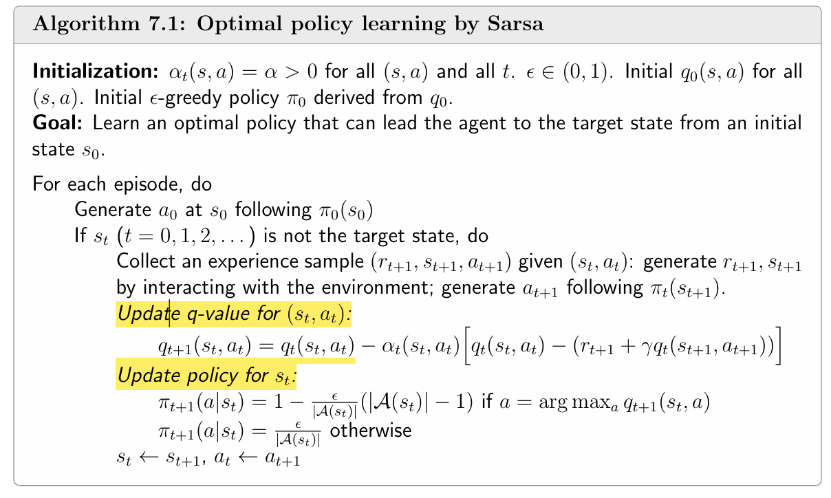
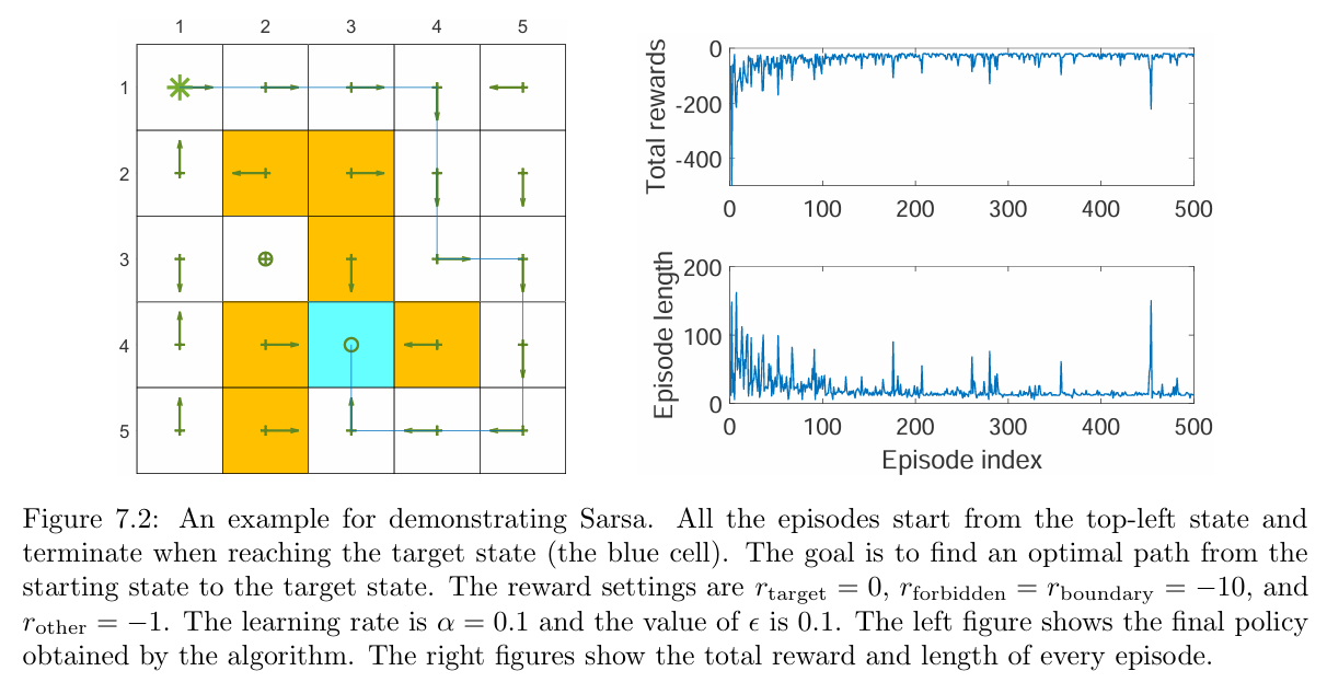
the total reward of each episode increases gradually. That is because the initial policy is not good and hence negative rewards are frequently obtained. As the policy becomes better, the total reward increases.
Notably, the length of an episode may increase abruptly (e.g., the 460th episode) and the corresponding total reward also drops sharply. That is because the policy is-greedy, and there is a chance for it to take non-optimal actions. One way to resolve this problem is to use decaying $\epsilon$ whose value converges to zero gradually(Gradually reduce $\epsilon$ or deal with smooth).
7.3 TD learning of action values : Expectded Sarsa
where $\mathbb{E}[q_{t}(s_{t+1},A)]=\sum_a\pi_t(a \mid s_{t+1})q_t(s_{t+1},a)=v_t(s_{t+1})$.
Since the algorithm involves an expected value, it is called Expected Sarsa. Although calculating the expected value may increase the computational complexity slightly, it is beneficial in the sense that it reduces the estimation variances because it reduces the random variables in Sarsa from ${s_t, a_t, r_{t+1}, s_{t+1}, a_{t+1}}$ to ${s_t, a_t, r_{t+1}, s_{t+1}}$ .
7.4 TD learning of action values : n-step Sarsa
The n-step Sarsa algorithm is a generalization of the Sarsa algorithm. It will be shown that Sarsa and MC learning are two special cases of n-step Sarsa.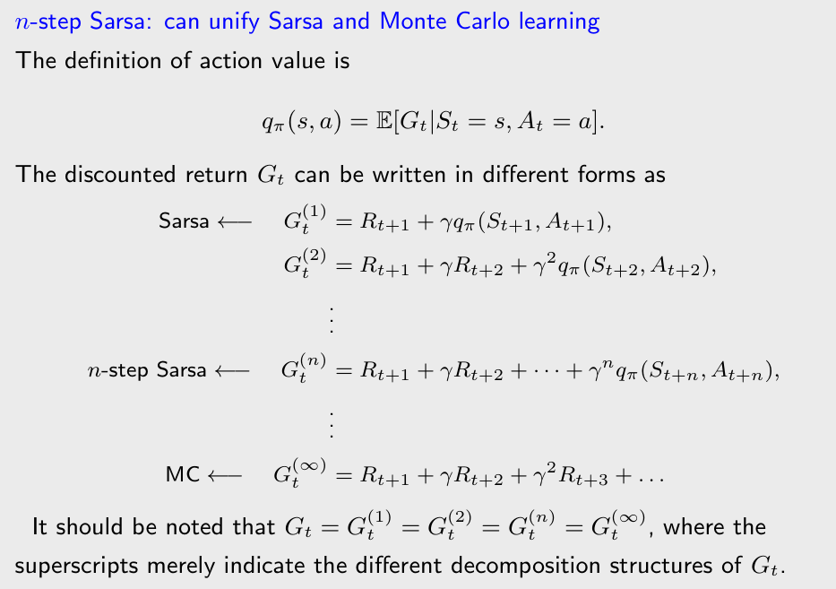
In summary, n-step Sarsa is a more general algorithm because it becomes the (one step) Sarsa algorithm when $n = 1$ and the MC learning algorithm when $n = \infty$(by setting $\alpha_t = 1$).
where $q_{t+n}(s_t, a_t)$ is the estimate of $q_{\pi}(s_t, a_t)$ at time $t + n$.
In particular, if $n$ is selected as a large number, n-step Sarsa is close to MC learning: the estimate has a relatively high variance but a small bias. If $n$ is selected to be small, n-step Sarsa is close to Sarsa: the estimate has a relatively large bias but a low variance.
7.5 TD learning of optimal action values : Q-Learning
The other TD algorithms aim to solve the Bellman equation of a given policy, Q-learning aims to directly solve the Bellman optimality equation to obtain optimal policies. Recall that Sarsa can only estimate the action values of a given policy, and it must be combined with a policy improvement step to find optimal policies. By contrast, Q-learning can directly estimate optimal action values and find optimal policies.
7.5.1 Algorithm description
The Q-learning algorithm is:
where $t = 0,1,2,\dots$ denotes the time step. Here, $q_t(s_t,a_t)$ is the estimate the optimal action value of (s_t,a_t) ; $\alpha_t(s_t,a_t)$ is the learning rate for $(s_t,a_t)$ at time $t$.
Q-learning is a stochastic approximation algorithm for solving the Bellman optimality equation expressed in terms of action values.
Sarsa requires $(r_{t+1}, s_{t+1}, a_{t+1})$ in every iteration, whereas Q-learning merely requires $(r_{t+1}, s_{t+1})$.
7.5.2 Off-policy and on-policy
Q-learning slightly special compared to the other TD algorithms is that Q-learning is off-policy while the others are on-policy.
Two policies exist in any reinforcement learning task: a behavior policy and a target policy.
- The behavior policy is the one used to generate experience samples.
- The target policy is the one that is constantly updated to converge to an optimal policy.
When the behavior policy is the same as the target policy, such a learning process is called on-policy. Otherwise, when they are different, the learning process is called off-policy.
The advantage of off-policy learning is that it can learn optimal policies based on the experience samples generated by other policies, which may be, for example, a policy executed by a human operator. As an important case, the behavior policy can be selected to be exploratory. For example, if we would like to estimate the action values of all state action pairs, we must generate episodes visiting every state-action pair sufficiently many times. Although Sarsa uses $\epsilon$-greedy policies to maintain certain exploration abilities, the value of is usually small and hence the exploration ability is limited. By contrast, if we can use a policy with a strong exploration ability to generate episodes and then use off-policy learning to learn optimal policies, the learning efficiency would be significantly increased.
Sarsa is on-policy.
we need samples generated by $\pi$. Therefore, $\pi$ is the behavior policy. The second step is to obtain an improved policy based on the estimated values of $\pi$. As a result, $\pi$ is the target policy that is constantly updated and eventually converges to an optimal policy. Therefore, the behavior policy and the target policy are the same.
Monte Carlo learning is on-policy.
A policy is used to generate samples, which is further used to estimate the action values of the policy. Based on the action values, we can improve the policy.
Q-learning is off-policy.
The fundamental reason is that Q-learning is an algorithm for solving the Bellman optimality equation that can directly generate the optimal values and optimal policies.we need not to evaluate the associated policy.
Q-learning experience sample requires $(s_t, a_t, r_{t+1},s_{t+1})$. If $(s_t, a_t)$ is given, then $r_{t+1}$ and $s_{t+1}$ do not depend on any policy!
The behavior policy to generate at from $s_t$ can be anything. The target policy will converge to the optimal policy.
Note: on-policy/off-policy is online/offline learning?
Online learning refers to the case where the value and the policy are updated once an experience sample is obtained. Offline learning refers to the case where the update can only be done after all experience samples have been collected(episodes).
7.5.3 Implementation and Illustrative examples
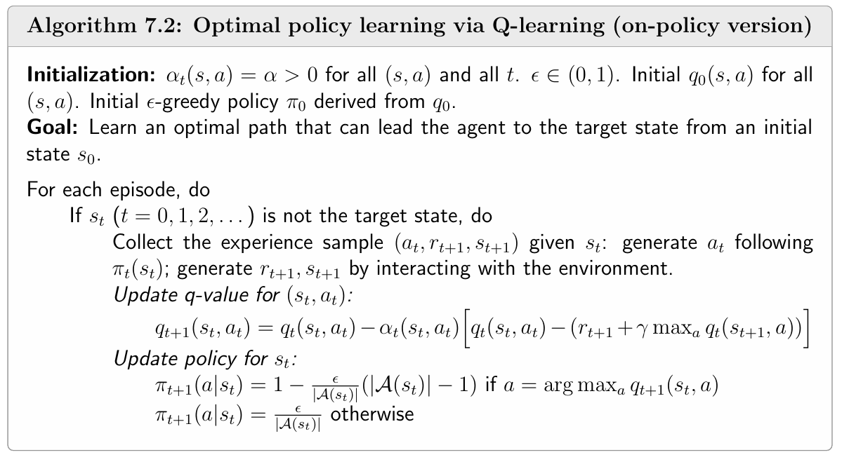
The on-policy version of Q-learning is shown in Algorithm 7.2. This implementation is similar to the Sarsa one in Algorithm 7.1. Here, the behavior policy is the same as the target policy, which is an-greedy policy.
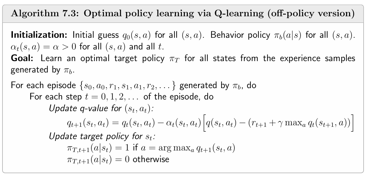
The off-policy version is shown in Algorithm 7.3. The behavior policy $\pi_b$ can be any policy as long as it can generate sufficient experience samples. It is usually favorable when $\pi_b$ is exploratory. Here, the target policy $\pi_T$ is greedy rather than $\epsilon$-greedy since it is not used to generate samples and hence is not required to be exploratory. Moreover, the off-policy version of Q-learning presented here is implemented offline: all the experience samples are collected first and then processed. It can be modified to become online: the value and policy can be updated immediately once a sample is received.
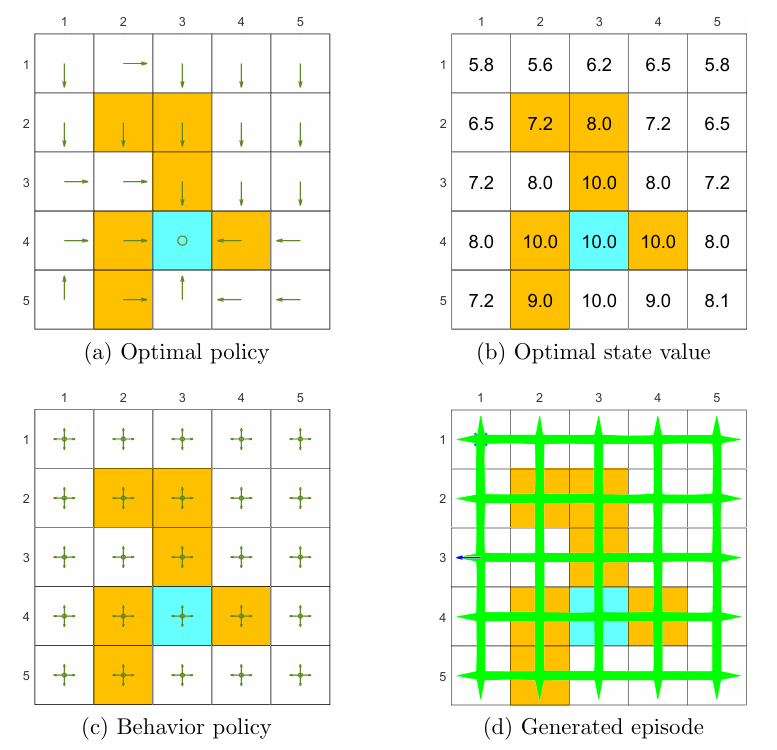
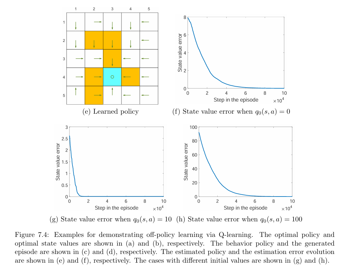
Ground truth: To verify the effectiveness of Q-learning, we first need to know the ground truth of the optimal policies and optimal state values. Here, the ground truth is obtained by the model-based policy iteration algorithm. The ground truth is given in Figures 7.4(a) and (b).
Experience samples: The behavior policy has a uniform distribution: the probability of taking any action at any state is 0.2 (Figure 7.4(c)). A single episode with 100,000 steps is generated (Figure 7.4(d)). Due to the good exploration ability of the behavior policy, the episode visits every state-action pair many times.
Learned results: Based on the episode generated by the behavior policy, the final target policy learned by Q-learning is shown in Figure 7.4(e). This policy is optimal because the estimated state value error (root-mean-square error) converges to zero as shown in Figure 7.4(f). In addition, one may notice that the learned optimal policy is not exactly the same as that in Figure 7.4(a). In fact, there exist multiple optimal policies that have the same optimal state values.
Different initial values: Since Q-learning bootstraps, the performance of the algorithm depends on the initial guess for the action values. As shown in Figure 7.4(g), when the initial guess is close to the true value, the estimate converges within approximately 10,000 steps. Otherwise, the convergence requires more steps (Figure 7.4(h)). Nevertheless, these figures demonstrate that Q-learning can still converge rapidly even though the initial value is not accurate.
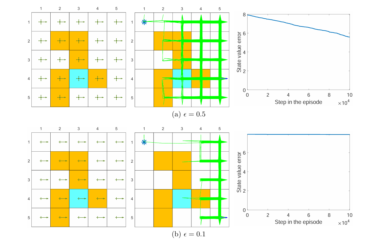
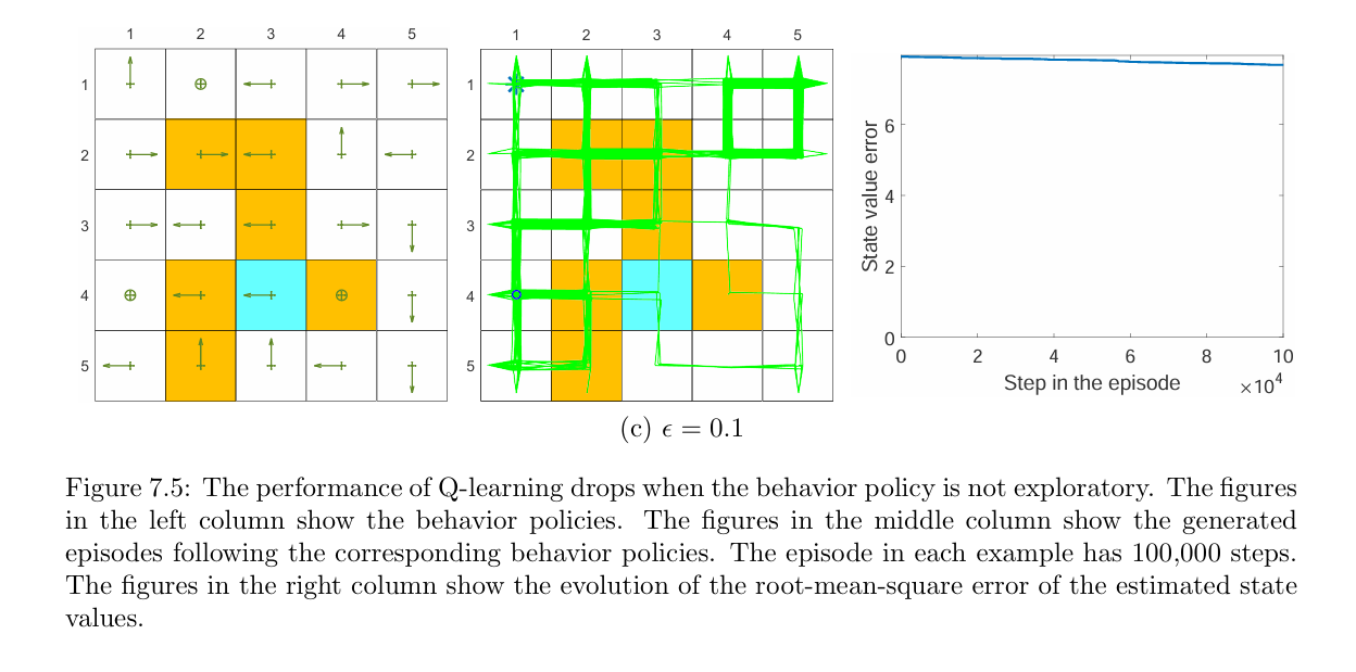
Different behavior policies: When the behavior policy is not exploratory, the learning performance drops significantly. For example, consider the behavior policies shown in Figure 7.5. They are $\epsilon$-greedy policies with = 0.5 or 0.1 (the uniform policy in Figure 7.4(c) can be viewed as $\epsilon$-greedy with = 1). It is shown that, when decreases from 1 to 0.5 and then to 0.1, the learning speed drops significantly. That is because the exploration ability of the policy is weak and hence the experience samples are insufficient.
7.6 A unified viewpoint
In this section, we introduce a uni ed framework to accommodate all these
algorithms and MC learning.
In particular, the TD algorithms (for action value estimation) can be expressed in a unified expression:
where $\bar{q_t}$ is the TD target. Different TD algorithms have different $\bar{q_t}$.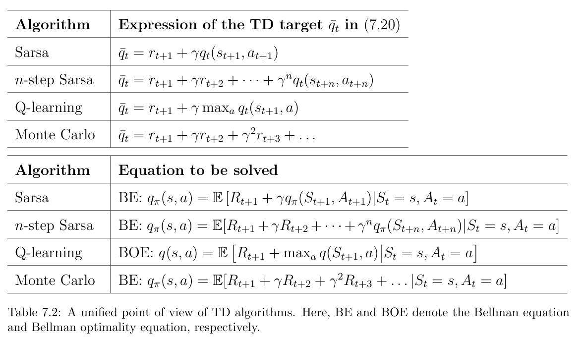
As can be seen, all of the algorithms aim to solve the Bellman equation except Q-learning, which aims to solve the Bellman optimality equation.
7.7 Summary
we introduced include Sarsa, n-step Sarsa, and Q-learning. All these algorithms can be viewed as stochastic approximation algorithms for solving Bellman or Bellman optimality equations.
The TD algorithms introduced in this chapter, except Q-learning, are used to evaluate a given policy. That is to estimate a given policy’s state/action values from some experience samples. Together with policy improvement, they can be used to learn optimal policies. Moreover, these algorithms are on-policy: the target policy is used as the behavior policy to generate experience samples.
Q-learning is slightly special compared to the other TD algorithms in the sense that it is o-policy. The target policy can be different from the behavior policy in Q-learning. The fundamental reason why Q-learning is o-policy is that Q-learning aims to solve the Bellman optimality equation rather than the Bellman equation of a given policy.
It is worth mentioning that there are some methods that can convert an on-policy algorithm to be off-policy. Importance sampling is a widely used one and will be introduced in Chapter 10. Finally, there are some variants and extensions of the TD algorithms introduced in this chapter 5. For example, the $TD(\lambda)$ method provides a more general and uni ed framework for TD learning. More information can be found in paper6.
5:H. Van Hasselt, A. Guez, and D. Silver, Deep reinforcement learning with double Q-learning, in AAAI Conference on Artificial Intelligence, vol. 30, 2016.
6:R. S. Sutton and A. G. Barto, Reinforcement learning: An introduction (2nd Edition). MIT Press, 2018.
Q: What does the term learning in TD learning mean?
A: From a mathematical point of view, learning simply means estimation . That is to estimate state/action values from some samples and then obtain policies based on the estimated values.
Q: Why does Sarsa update policies to be-greedy?
A: That is because the policy is also used to generate samples for value estimation. Hence, it should be exploratory to generate sufficient experience samples.
Q: While Theorems 7.1 and 7.2 require that the learning rate t converges to zero gradually, why is it often set to be a small constant in practice?
A: The fundamental reason is that the policy to be evaluated keeps changing (or called nonstationary). In particular, a TD learning algorithm like Sarsa aims to estimate the action values of a given policy. If the policy is fixed, using a decaying learning rate is acceptable. However, in the optimal policy learning process, the policy that Sarsa aims to evaluate keeps changing after every iteration. We need a constant learning rate in this case; otherwise, a decaying learning rate may be too small to effectively evaluate policies. Although a drawback of constant learning rates is that the value estimate may fluctuate eventually, the fluctuation is negatable as long as the constant learning rate is sufficiently small.
Q: Why does the o-policy version of Q-learning update policies to be greedy instead of $\epsilon$-greedy?
A: That is because the target policy is not required to generate experience samples. Hence, it is not required to be exploratory.
Approximation (Q-learning Steps)
The Q-learning algorithm uses a Q-table of State-Action Values (also called Q-values). This Q-table has a row for each state and a column for each action. Each cell contains the estimated Q-value for the corresponding state-action pair.
Steps:
1.We start by initializing all the Q-values to zero. As the agent interacts with the environment and gets feedback, the algorithm iteratively improves these Q-values until they converge to the Optimal Q-values. It updates them using the Bellman equation.
2.Then we use the ε-greedy policy to pick the current action from the current state.
3.Execute this action tointhe environment to execute, and gets feedback in the form of a reward and the next state.
4.Now, for step #4, the algorithm has to use a Q-value from the next state in order to update its estimated Q-value (Q1) for the current state and selected action.
And here is where the Q-Learning algorithm uses its clever trick. The next state has several actions, so which Q-value does it use? It uses the action (a4) from the next state which has the highest Q-value (Q4). What is critical to note is that it treats this action as a target action to be used only for the update to Q1. It is not necessarily the action that it will actually end up executing from the next state when it reaches the next time step.
Here $d_t$ is the done flag. If $d_t=1$, then it means the state $s_{t+1}$ is a terminal state. Adding the $\left(1-d_t\right)$ term implies that the discounted return $G_t$ is just going to be $r_t$, since all rewards after that are going to be 0 . In some situations this can help accelerate learning.
In other words, there are two actions involved:
- Current action — the action from the current state that is actually executed in the environment, and whose Q-value is updated.
- Target action — has the highest Q-value from the next state, and used to update the current action’s Q value.