Mathematical Foundation of Reinforcement Learning-DQN algorithm

[toc]

Sources:

1. Shiyu Zhao. 《Mathematical Foundation of Reinforcement Learning》Chapter 8.
2. OpenAI Spinning Up

8 Value Function Approximation

we continue to study temporal-difference learning algorithms. However, a different method is used to represent state/action values. The tabular method(Q-learning) is straight forward to understand, but it is inefficient for handling large state or action spaces. To solve this problem, this chapter introduces the function approximation method, which has become the standard way to represent values. It is also where artificial neural networks are incorporated into reinforcement learning as function approximates. The idea of function approximation can also be extended from representing values to representing policies, as introduced in Chapter 9.

8.1 Value representation: From table to function

The tabular method

state	$s_1$	$s_2$	…	$s_n$
Estimated value	$\hat{v}(s_1)$	$\hat{v}(s_2)$	…	$\hat{v}(s_1)$

Q-learning	$a_1$	$a_2$	…	$a_m$
$s_1$	$q_(s_1,a_1)$	$q_(s_1,a_2)$	…	$q_(s_1,a_m)$
$s_2$	$q_(s_2,a_1)$	$q_(s_2,a_2)$	…	$q_(s_2,a_m)$
…	…	…	…	…
$s_n$	$q_(s_n,a_1)$	$q_(s_n,a_2)$	…	$q_(s_n,a_m)$

The function approximation method (for example approximated by a straight line)

$$\hat{v}(s,w) = as+b=\underbrace{[s,1]}_{\phi^T(s)}\underbrace{\begin{bmatrix} a \\ b \\ \end{bmatrix}}_{w}= \phi^T(s)w. \tag{8.1}$$

Here, $\hat{v}(s,w)$ is a function for approximating $v_{\pi}(s)$. It is determined jointly by the state $s$ and the parameter vector $w \in \mathbb{R}^2$. $\hat{v}(s,w)$ is sometimes written as $\hat{v}_w(s)$. Here, $\phi(s)\in \mathbb{R}^2$ is called the feature vector of $s$.

tabular method	function approximation	compared anlysis
retrieve a value: directly read the corresponding entry in the table.	retrieve a value: input the state index s into the function and calculate the function value	The function approximation method enhances storage efficiency by sacrificing accuracy.
update a value: directly rewrite the corresponding entry in the table.	update a value : update $w$ to change the values indirectly.	the function approximation method has another merit: its generalization ability is stronger than that of the tabular method.

efficient: The function approximation method is only need to store a lower dimensional parameter vector $w$. however, not free. It comes with a cost: the state values may not be accurately represented by the function.

generalization ability: When using the tabular method, we can update
a value if the corresponding state is visited in an episode. The values of the states that have not been visited cannot be updated. However, when using the function approximation method, we need to update $w$ to update the value of a state. The update of $w$ also affects the values of some other states even though these states have not been visited. Therefore, the experience sample for one state can generalize to help estimate the values of some other states. The above analysis is illustrated in blow Figure.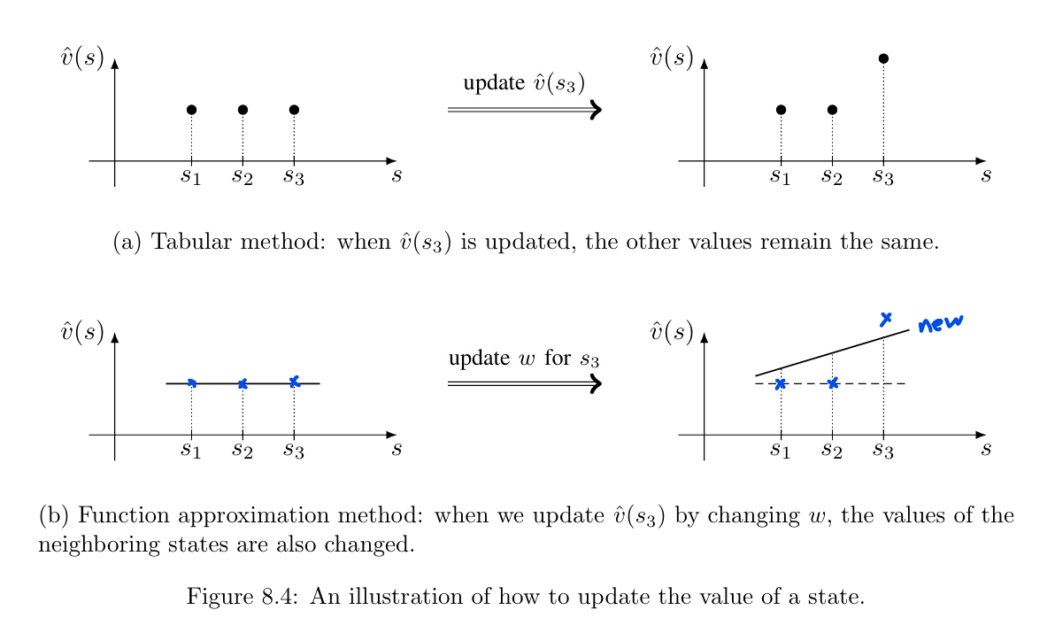

We can use more complex functions that have stronger approximation abilities than straight lines. For example, consider a second-order polynomial:

$$\hat{v}(s,w) = as^2+bs+c=\underbrace{[s^2,s,1]}_{\phi^T(s)}\underbrace{\begin{bmatrix} a \\ b \\ c \\ \end{bmatrix}}_{w}= \phi^T(s)w. \tag{8.2}$$

Note that $\hat{v}(s,w)$ in either (1) or (2) is linear in $w$ (though it may be nonlinear in $s$). This type of method is called linear function approximation, which is the simplest function approximation method. To realize linear function approximation, The basis is to select an appropriate feature vector $\phi(s)$. It requires prior knowledge of the given task: the better we understand the task, the better the feature vectors we can select. However, such prior knowledge is usually unknown in practice. If we do not have any prior knowledge,a popular solution is to use artificial neural networks as nonlinear function approximations.

The chapter’s key is how to find the optimal parameter vector $w$.. If we know $v_{\pi}(s_i)$(the real value), this is a least-squares problem. The optimal parameter can be obtained by optimizing the following objective function:

$$J_1 =\sum_{i=1}^n(\hat{v}(s_i,w)-v_{\pi}(s_i))^2=\sum_{i=1}^n(\phi^T(s_i)w-v_{\pi}(s_i))^2$$

8.2 TD learning of state values based on function approximation

how to integrate the function approximation method into TD learning to estimate the state values(the based TD algorithm) of a given policy.This algorithm will be extended to learn action values (sarsa) and optimal policies (Q-learning) in Section 8.3. Therefore,this section is the foundation of section 8.3.

Key core of this chapter：**How to find the optimal parameter vector $w$? == How to update the state/action value?**
The function approximation method is formulated as an optimization problem.
(1) The objective function of this problem is introduced in Section 8.2.1 (the loss function).
(2) The TD learning algorithm for optimizing this objective function is introduced in Section 8.2.2. (the optimal algorithm:SGD and TD learning algorithm)
(3) There are two ways to formulate value function $\hat{v}(s,w)$/$\hat{q}(s,a,w)$ (formulate affine model).

• 3.1) TD-Linear: use a linear function,we need to select appropriate feature vectors. (Section 8.2.3: the based TD algorithm; section 8.3: sarsa\Q-learning);
• 3.2) Artificial neural network as a nonlinear function approximate (Section 8.4: DQN).

8.2.1 Objective function

The problem to be solved is to find an optimal $w$ so that $\hat{v}(s,w)$ can best approximate $v_{\pi}(s)$ for every s. In particular, the objective function is

$$J(w) =\mathbf{E}[(v_{\pi}(S)-\hat{v}(S,w))^2] \tag{8.3}$$

While $S$ is a random variable, what is its probability distribution? There are several ways to define the probability distribution of $S$:

(1) The first way is to use a uniform distribution：(setting the probability of each state to $1/n$.)

$$J(w) =\mathbf{E}[(v_{\pi}(S)-\hat{v}(S,w))^2]= \frac{1}{n} \sum_{s \in S}(v_{\pi}(s)-\hat{v}(s,w))^2$$

which is the average value of the approximation errors of all the states. However, this way does not consider the real dynamics of the Markov process under the given policy. Since some states may be rarely visited by a policy, it may be unreasonable to treat all the states as equally important.

(2) The second way is to use the stationary distribution：(setting the probability of each state to the frequency of agent access to the state.)

The stationary distribution describes the long-term behavior of a Markov decision process. More specifically, after the agent executes a given policy for a sufficiently long period, the probability of the agent being located at any state can be described by this stationary distribution.

$$J(w) =\mathbf{E}[(v_{\pi}(S)-\hat{v}(S,w))^2]= \sum_{s \in S}d_{\pi}(s)(v_{\pi}(s)-\hat{v}(s,w))^2$$

which $d_{\pi}(s)$ denote the stationary distribution of the Markov process under policy $\pi$. $\sum_{s \in S}d_{\pi}(s)=1$.

it was assumed that the number of states was finite in the above equation. When the state space is continuous, we can replace the summations with integrals.

It is notable that the value of $d_{\pi}(s)$ is nontrivial to obtain because it requires knowing the state transition probability matrix $P_{\pi}$. Fortunately, we do not need to calculate the specific value of $d_{\pi}(s)$ to minimize this objective function as shown in the next subsection. I.e. When optimizing based on gradient descent, the experience samples are collected by the behavior strategy, which inherently have the meaning of $d_{\pi}(s)$.

Conditions for the uniqueness of stationary distributions.
A general class of Markov processes that have unique stationary(or limiting)distributions is irreducible(or regular) Markov processes.
— A Markov process is called irreducible if all of its states communicate with each other.
— A Markov process is called regular if there exists $k >=1$ such that $[P_{\pi}]_{ij}^k>0$ for all $i,j$. States $j$ is said to be accessible from state $s_i$ if there exists a finite integer $k$ so that $[P_{\pi}]_{ij}^k>0$

Policies that may lead to unique stationary distributions.
Once the policy is given, a Markov decision process becomes a Markov process, whose long-term behavior is jointly determined by the given policy and the system model. Then,an important question is what kind of policies can lead to regular Markov processes? In general,the answer is exploratory policies such as $\epsilon$-greedy policies. I.e.,since all the states communicate,there sulting Markov process is irreducible. Second, since every state can transition to itself, there resulting Markov process is regular.
— application —
There are two methods to calculate the stationary distributions.
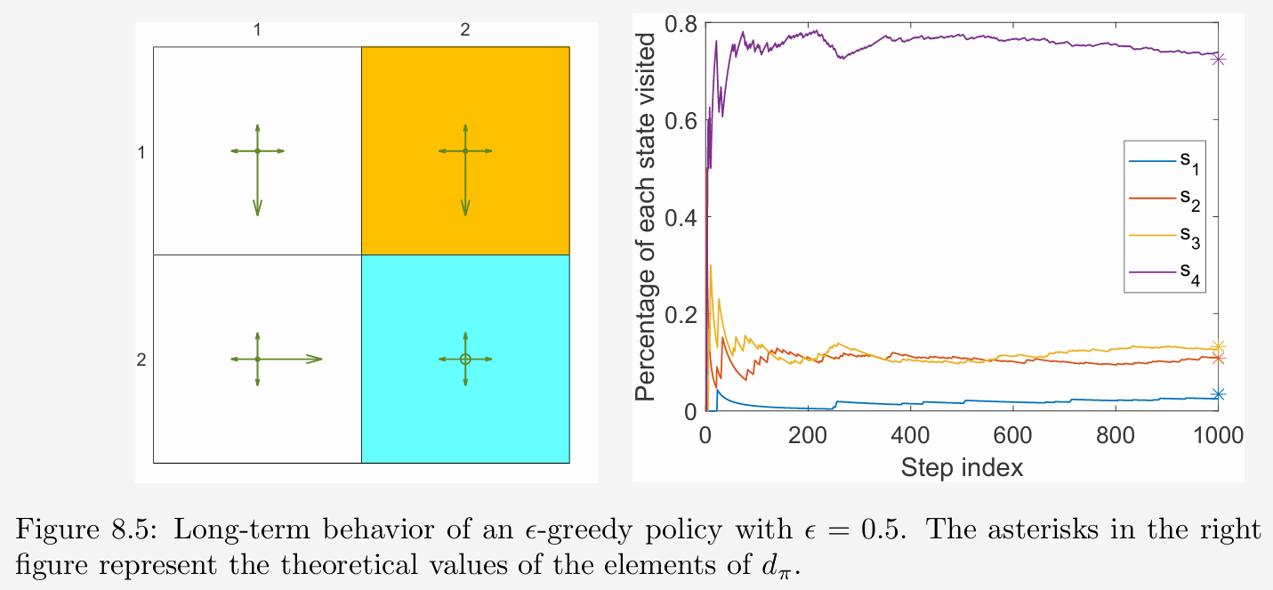
— (1) The theoretical value of $d_{\pi}$ can be calculated by the state transition probability matrix $P_{\pi}$.
— (2) The second method is to estimated $d_{\pi}$ numerically. we start from an arbitrary initial state and generate a sufficiently long episode by following the given policy. we select $s_1$ as the starting state and run 1000 steps by following the policy. The proportion of the visits of each state during the process is shown in the below Figure( represent the theoretical value of $d_{\pi}(s_i)$). *It can be seen that the proportions converge to the theoretical value of $d_{\pi}$ after hundreds of steps. It is clear clarify that the experience samples are collected by the behavior strategy, which inherently have the meaning of $d_{\pi}(s)$.

8.2.2 Optimization algorithms

To minimize the objective function $J(w)$, we can use the gradient descent algorithm:

$$w_{k+1}=w_k - \alpha_{k} \nabla_{w} J(w_k),$$

where

$$\begin{aligned} \nabla_{w} J(w_k) &=\nabla_{w} \mathbb{E}[(v_{\pi}(S)-\hat{v}(S,w_k))^2] \\ & =\mathbb{E}[\nabla_{w}(v_{\pi}(S)-\hat{v}(S,w_k))^2]\\ & =2\mathbb{E}[\nabla_{w}(v_{\pi}(S)-\hat{v}(S,w_k))(-\nabla_{w}\hat{v}(S,w_k))]\\ & =-2\mathbb{E}[\nabla_{w}(v_{\pi}(S)-\hat{v}(S,w_k))\nabla_{w}\hat{v}(S,w_k)] \end{aligned}$$

Therefore, the gradient descent algorithm is

$$w_{k+1}=w_k +2\alpha_{k}\mathbb{E}[(v_{\pi}(S)-\hat{v}(S,w_k))\nabla_{w}\hat{v}(S,w_k)], \tag{8.4}$$

where the coefficient 2 before $\alpha_{k}$ can be merged into $\alpha_{k}$ without loss of generality. In the spirit of stochastic gradient descent, we can replace the true gradient with a stochastic gradient. Then, becomes

$$w_{t+1}=w_t +\alpha_{t}(v_{\pi}(s_t)-\hat{v}(s_t,w_t))\nabla_{w}\hat{v}(s_t,w_t), \tag{8.5}$$

where $s_t$ is a sample of $S$ at time $t$. Notably, this equation is not implementable because it requires the true state value $v_{\pi}$ , which is unknown and must be estimated.

The following two methods can replace $v_{\pi}(s_t)$ with an approximation to make the algorithm implementable.
—— Monte Carlo method: Suppose that we have an episode $(s_0,r_1,s_1, r_2
\dots )$. Let $g_t$ be the discounted return starting from $s_t$. Then, $g_t$ can be used as an approximation of $v_{\pi} (s_t)$. The algorithm of Monte Carlo learning with function approximation becomes

$$w_{t+1}=w_t +\alpha_{t}(\textcolor{red}{g_t}-\hat{v}(s_t,w_t))\nabla_{w}\hat{v}(s_t,w_t), \tag{8.6}$$

—— Temporal-difference method: In the spirit of TD learning, $r_{t+1} + \gamma \hat{v}(s_{t+1},w_t)$ can be used as an approximation of $v_{\pi} (s_t)$. The algorithm of TD learning with function approximation becomes

$$w_{t+1}=w_t +\alpha_{t}(\overbrace{\textcolor{red}{\underbrace{r_{t+1} + \gamma \hat{v}(s_{t+1},w_t)}_{TD \ \ target}}-\hat{v}(s_t,w_t)}^{TD \ \ error})\nabla_{w}\hat{v}(s_t,w_t), \tag{8.7}$$

Understanding the TD learning with function approximation is important for studying the section 8.3. Notably, this equation can only learn the state values of a given policy. It will be extended to algorithms that can learn action values in Sections 8.3.

8.2.3 TD-Linear approximates（select appropriate feature vectors）

The linear function:

$$\hat{v}(s,w) = \phi^T(s)w.$$

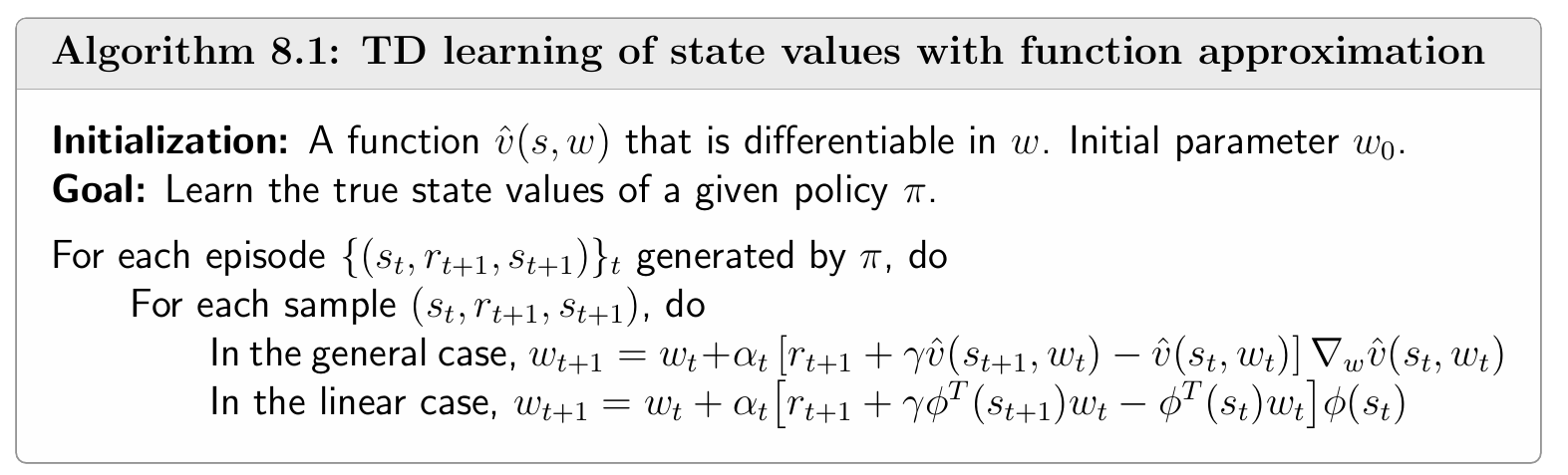
where $\phi(s) \in \mathbb{R}^m$ is the feature vector of $s$. The lengths of $\phi(s)$ and $w$ are equal to $m$, which is usually much smaller than the number of states. In the linear case, the gradient is $\nabla_{w}\hat{v}(s,w_k)=\phi(s)$.

This is the algorithm of TD learning with linear function approximation. We call it TD-Linear for short.

The linear case is much better understood in theory than the nonlinear case. However, its approximation ability is limited. It is also nontrivial to select appropriate feature vectors for complex tasks. By contrast, artificial neural networks can approximate values as black-box universal nonlinear approximates, which are more friendly to use.

The reason is to learn TD-linear that a better understanding of the linear case can help readers better grasp the idea of the function approximation method. More importantly, the linear case is still powerful in the sense that the tabular method can be viewed as a special linear case.

Tabular TD learning is a special case of TD-Linear.
Consider the following special feature vector for any $s\in S$:

$$\phi(s)=e_s \in \mathbb{R}^n$$

where $e_s$ is the vector with the entry corresponding to s equal to 1,and the others as 0. In this case,

$$\hat{v}(s,w) = e_s^Tw = w(s).$$

where $w(s)$ is the $s$th entry of $w$.

$$\begin{aligned} w_{t+1} &=w_t +\alpha_{t}(r_{t+1} + \gamma \hat{v}(s_{t+1},w_t)-\hat{v}(s_t,w_t))\phi(s_t)\\ &=w_t +\alpha_{t}(r_{t+1} + \gamma w_t(s_{t+1})-w_t(s_t))e_{s_t}\\ &=w_t +\alpha_{t}(r_{t+1} + \gamma w_t(s_{t+1})-w_t(s_t)), \end{aligned}$$

which is exactly the tabular TD algorithm.

We next present some examples for demonstrating how to use the TD-Linear algorithm to estimate the state values of a given policy? . In the meantime, we demonstrate how to select feature vectors?

The grid world example is shown in the below Figure 8.6. The given policy takes any action at a state with a probability of 0.2(exploratory). Our goal is to estimate the state values under this policy. There are 25 state values in total. The true state values are shown in Figure 8.6(b). The true state values are visualized as a three-dimensional surface in Figure 8.6(c)

We next show that we can use fewer than 25 parameters to approximate these state values. The simulation setup is as follows. Five hundred episodes are generated by the given policy. Each episode has 500 steps and starts from a randomly selected state-action pair following a uniform distribution. In addition, in each simulation trial, the parameter vector $w$ is randomly initialized such that each element is drawn from a standard normal distribution with a zero mean and a standard deviation of 1. We set $r_{forbidden} = r_{boundary} = -1, r_{target} = 1$, and $\gamma = 0.9$.

To implement the TD-Linear algorithm, we need to select the feature vector $\phi(s)$ first. There are different ways to do that as shown below.

— (1) The first type of feature vector is based on polynomials. In the grid world example, a state $s$ corresponds to a 2D location. Let $x$ and $y$ denote the column and row indexes of $s$, respectively. To avoid numerical issues, we normalize x and y so that their values are within the interval of $[-1,+1]$.

$$\begin{aligned} &\phi(s)=\begin{bmatrix} a \\ b \\ \end{bmatrix} \in \mathbb{R}^2,\\ &\hat{v}(s,w)=\phi^T(s)w=[x,y]\begin{bmatrix} w_1 \\ w_2 \\ \end{bmatrix}=w_1x+w_2y. \end{aligned}$$

When $w$ is given, $\hat{v}(s,w) = w_1x+w_2y$ represents a 2D plane that passes through the origin. Since the surface of the state values may not pass through the origin, we need to introduce a bias to the 2D plane to better approximate the state values. In this case, the approximated state value is

$$\begin{aligned} \hat{v}(s,w)=\phi^T(s)w=[1,x,y]\begin{bmatrix} w_1\\ w_2 \\ w_3 \\ \end{bmatrix}=w_1+w_2x+w_2y. \end{aligned}$$

The estimation result when we use the feature vector in $[1,x,y]$ is shown in Figure 8.7(a). Although the estimation error converges as more episodes are used, the error cannot decrease to zero due to the limited approximation ability of a 2D plane.
To enhance the approximation ability, we can increase the dimension of the feature vector.
a quadratic 3D surface: (in Figures 8.7(b))

$$\phi(s)=[1,x,y,x^2,y^2,xy]^T \in \mathbb{R}^6$$

a cubic 3D surface: (in Figures 8.7(c))

$$\phi(s)=[1,x,y,x^2,y^2,xy,x^3,y^3,x^2y,xy^2]^T \in \mathbb{R}^{10}$$

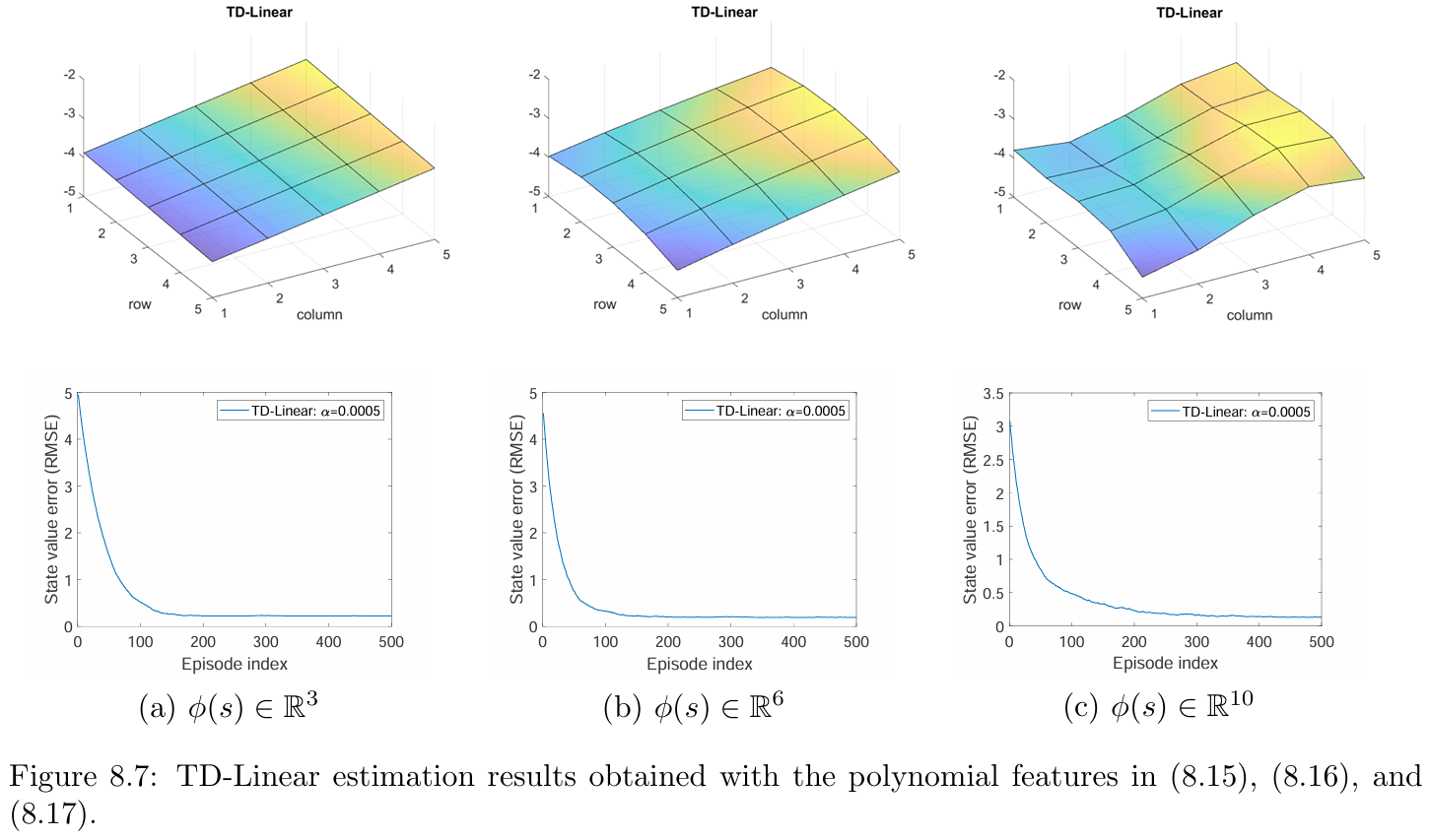
As can be seen, the longer the feature vector is, the more accurately the state values can be approximated. However, in all three cases, the estimation error cannot converge to zero because these linear approximates still have limited approximation abilities.

— (2) The others type of feature vector such as Fourier basis and tile coding. First, the values of $x$ and $y$ of each state are normalized to the interval of $[0,1]$. The resulting feature vector is

$$\phi(s)=\begin{bmatrix} \vdots\\ cos(\pi(c_1x+c_2y)) \\ \vdots \\ \end{bmatrix} \in \mathbb{R}^{(q+1)^2},$$

where $\pi$ denotes the circumference ratio,which is $3.1415\dots$ ,instead of a policy. $c_1$ or $c_2$ can be set as any integers in ${0,1,\dots,q}$,where $q$ is a user-specified integer. As a result, there are $(q+1)^2$ possible values for the pair $(c_1 c_2)$ to take. For example, in the case of $q=1$, the feature vector is

$$\phi(s)=\begin{bmatrix} cos(\pi(0x+0y))\\ cos(\pi(0x+1y)) \\ cos(\pi(1x+0y)) \\cos(\pi(1x+1y))\\ \end{bmatrix}= \begin{bmatrix} 1\\ cos(\pi y) \\ cos(\pi x) \\cos(\pi(x+y))\\ \end{bmatrix}\in \mathbb{R}^{4},$$

The estimation results obtained when we use the Fourier features with $q=1,2,3$ are shown in Figure 8.8. As can be seen, the higher the dimension of the feature vector is, the more accurately the state values can be approximated.

8.2.4 Theoretical analysis of TD-Linear approximates

The algorithm

$$w_{t+1}=w_t +\alpha_{t}(\textcolor{red}{r_{t+1} + \gamma \hat{v}(s_{t+1},w_t)}-\hat{v}(s_t,w_t))\nabla_{w}\hat{v}(s_t,w_t),$$

does not minimize the following objective function:

$$J(w) =\mathbb{E}[(v_{\pi}(S)-\hat{v}(S,w))^2]$$

Different objective functions:
Objective function 1: True value error

$$J_E(w) =\mathbb{E}[(v_{\pi}(S)-\hat{v}(S,w))^2]=||\hat{v}(w)-v_{\pi}||^2_D$$

Objective function 2: Bellman error

$$J_E(w) =||\hat{v}(w)-(r_{\pi}+\gamma P_{\pi}\hat{v}(w))||^2_D=||\hat{v}(w)-T_{\pi}(\hat{v}(w))||^2_D$$

where $T_{\pi}(x) = r_{\pi} + \gamma P_{\pi}x $

Objective function 3: Projected Bellman error

$$J_PBE(w) =||\hat{v}(w)-MT_{\pi}(\hat{v}(w))||^2_D$$

where $M$ is a projection matrix.
The TD-Linear algorithm minimizes the projected Bellman error. we can always find a value of $w$ that can minimize $J_{PBE}(w)$ to zero. Like the TD-Linear algorithm, least-squares TD algorithm (LSTD) aims to minimize the projected Bellman error. But TD algorithm and LSTD obtain the estimated value $\hat{v}(w)$ also close the true state value $v_{\pi}$ . Details can be found in the book.

8.3 TD learning of action values based on function approximation

the present section introduces how to estimate action values. The tabular Sarsa and tabular Q-learning algorithms are extended to the case of value function approximation. Readers will see that the extension is straightforward.

8.3.1 Sarsa with function approximation

The Sarsa algorithm with function approximation can be readily by replacing the state values with action values.

$$w_{t+1}=w_t +\alpha_{t}(r_{t+1} + \gamma \textcolor{red}{\hat{q}(s_{t+1},a_{t+1},w_t)}-\textcolor{red}{\hat{q}(s_t,a_t,w_t)})\nabla_{w}\textcolor{red}{\hat{q}(s_t,a_t,w_t)}. \tag{8.8}$$

When linear functions are used, we have $\hat{q}(s_t,a_t,w_t)=\phi^T(s,a)w$ where $\phi(s,a)$ is a feature vector.
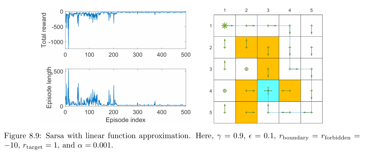
The value estimation step in the equation can be combined with a policy improvement step to learn optimal policies. The procedure is summarized in Algorithm 8.2. It is notable that this equation is executed only once before switching to the policy improvement step. This is similar to the tabular Sarsa algorithm.
Moreover, the implementation in Algorithm 8.2 aims to solve the task of finding a good path to the target state from a presanctified starting state. As a result, it cannot find the optimal policy for every state. However, if sufficient experience data are available, the implementation process can be easily adapted to find optimal policies for every state.

An illustrative example is shown in Figure 8.9. In this example, the task is to find a good policy that can lead the agent to the target when starting from the top-left state. Both the total reward and the length of each episode gradually converge to steady values. In this example, the linear feature vector is selected as the Fourier function of order 5. The expression of a Fourier feature vector is given in the above equation.

8.3.2 Q-learning with function approximation

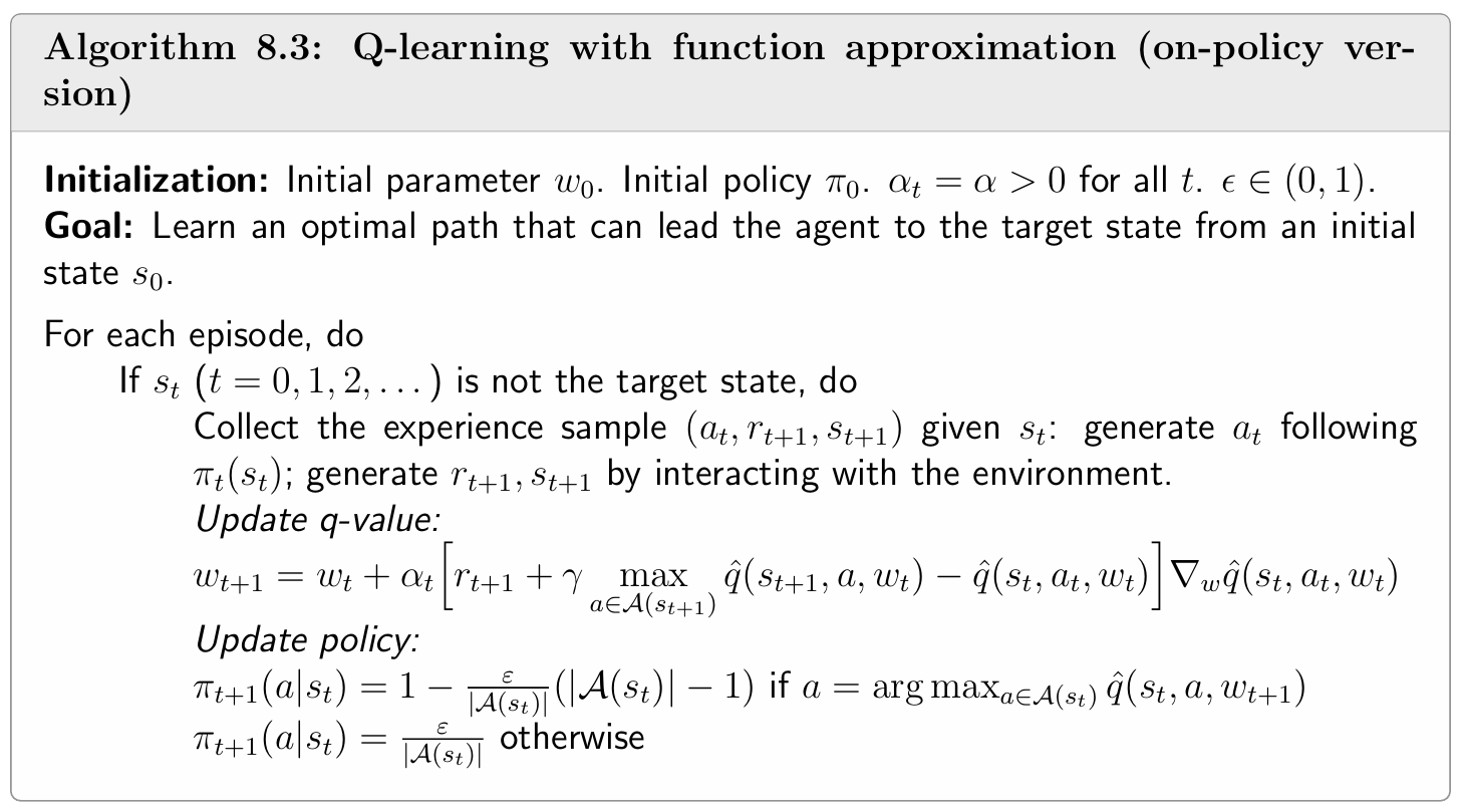
Tabular Q-learning can also be extended to the case of function approximation. The update rule is

$$w_{t+1}=w_t +\alpha_{t}(\textcolor{red}{r_{t+1}+\gamma \max_{a \in \mathbb{A}(s_{t+1})}q_{t}(s_{t+1},a_{t+1},w_t)}-\hat{q}(s_t,a_t,w_t))\nabla_{w}\hat{q}(s_t,a_t,w_t). \tag{8.9}$$

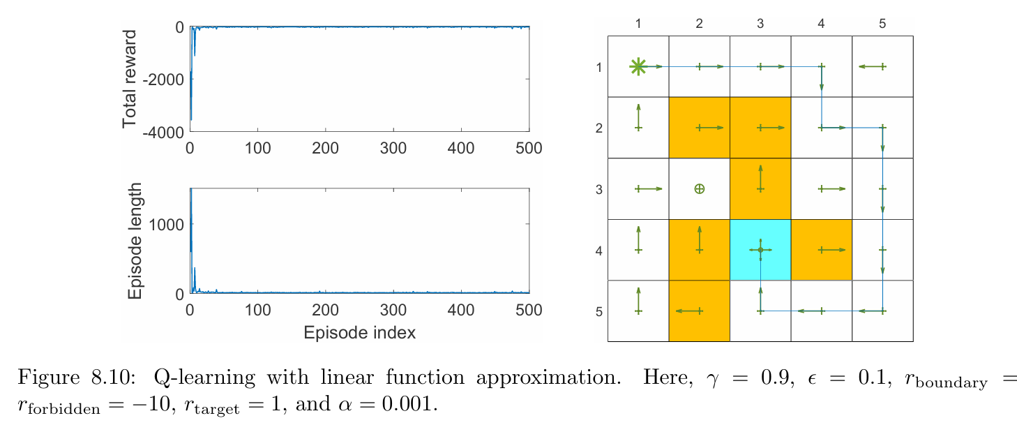
An on-policy version is given in Algorithm 8.3. An example for demonstrating the on-policy version is shown in Figure 8.10. In this example, the task is to find a good policy that can lead the agent to the target state from the top-left state.

As can be seen, Q-learning with linear function approximation can successfully learn an optimal policy. Here, linear Fourier basis functions of order five are used. The off-policy version will be demonstrated when we introduce deep Q-learning in Section 8.4.

One may notice in Algorithm 8.2 and Algorithm 8.3 that, although the values are represented as functions, the policy $\pi(a|s)$ is still represented as a table. Thus, it still assumes nite numbers of states and actions. In Chapter 9, we will see that the policies can be represented as functions so that continuous state and action spaces can be handled.

8.4 Deep Q-learning

We can integrate deep neural networks into Q-learning to obtain an approach called deep Q-learning or deep Q-network (DQN) ¹. Deep Q-learning is one of the earliest and most successful deep reinforcement learning algorithms. Notably, the neural networks do not have to be deep. For simple tasks such as our grid world examples, shallow networks with one or two hidden layers may be sufficient.
Deep Q-learning can be viewed as an extension of the Q-learning algorithm in section 8.3. However, its mathematical formulation and implementation techniques are substantially different and deserve special attention.

¹. V. Mnih, K. Kavukcuoglu, D. Silver, A. A. Rusu, J. Veness, M. G. Bellemare, A. Graves, M. Riedmiller, A. K. Fidjeland, G. Ostrovski, S. Petersen, C. Beattie, A. Sadik, I. Antonoglou, H. King, D. Kumaran, D. Wierstra, S. Legg, and D. Hassabis, Human-level control through deep reinforcement learning, Nature, vol. 518, ↩

no. 7540, pp. 529533, 2015.

8.4.1 Algorithm description

Mathematically, deep Q-learning aims to minimize the following objective function:

$$J=\mathbb{E}\left[\left(R+\gamma \max_{a \in \mathbb{A}(s^{\prime})}q_{t}(S^{\prime},a,w)-\hat{q}(S,A,w)\right)^2\right]. \tag{8.10}$$

where $(S,A,R,S^{\prime})$ are random variables that denote a state, an action, the immediate reward, and the next state, respectively. This objective function can be viewed as the squared Bellman optimality error.

To minimize the objective function in below equation, we can use the gradient descent algorithm to calculate the gradient of $J$ with respect to $w$. It is noted that the parameter $w$ appears not only in $\hat{q}(S,A,w)$ but also in $y = R+\gamma \max_{a \in \mathbb{A}(s^{\prime})}q_{t}(S^{\prime},a,w)$. it is nontrivial to calculate the gradient. For the sake of simplicity, it is assumed that the value of $w$ in $y$ is fixed (for a short period of time) so that the calculation of the gradient becomes much easier. In particular, we introduce two networks: one is a main network representing $\hat{q}(s,a,w)$ and the other is a target network $\hat{q}(s,a,w_T)$. The objective function in this case become

$$J=\mathbb{E}\left[\left(R+\gamma \max_{a \in \mathbb{A}(s^{\prime})}q_{t}(S^{\prime},a,\textcolor{red}{w_T})-\hat{q}(S,A,w)\right)^2\right].$$

where $w_T$ is the target networks parameter. When $w_T$ is fixed, the gradient of $J$ is

$$\nabla_wJ=-\mathbb{E}\left[\left(R+\gamma \max_{a \in \mathbb{A}(s^{\prime})}q_{t}(S^{\prime},a,w_T)-\hat{q}(S,A,w)\right)\nabla_w\hat{q}(S,A,w)\right]. \tag{8.11}$$

where some constant coefficients are omitted without loss of generality. The use of this gradient be hidden in the optimizer of Pytorch environment(the software tools for training neural networks).

The two most important characteristics of DQN:
(1) Two networks: a main network and a target network.
Let $w$ and $w_T$ denote the parameters of the main and target networks, respectively. They are initially set to the same value.The main network is updated in every iteration. By contrast, the target network is set to be the same as the main network every certain number of iterations to satisfy the assumption that $w_T$ is fixed when calculating the gradient in (11).
TD target changes after each update, thereby the entire training process is like chasing a moving target.

Deep Q-Learning算法解决了tabular
Q-Learning算法状态空间过大时造成的维度灾难/存储空间爆炸的问题。DQN算法中引入了深度神经网络来近似Q值函数，通过经验回放和‘目标网络-主网络’的双网络训练方式来提高算法的稳定性和收敛性。

• 经验回放：通过从经验池中均匀随机采样构造训练样本批次，来满足常用的MSE损失函数要求的均匀分布假设。（否则采样过程服从‘稳态分布’（stationary distribution）。）
• 目标网络-主网络：通过固定目标网络的参数，减少目标值的波动，提高算法的稳定性。

注：书中讲解此处时，是通过‘max’函数难以求导的问题引出的，我个人认为这是一个较容易理解的方式，但是认为这并不是‘双网络’最大的优势（回想在卷积神经网络中的最大池化操作是如何通过bp求导的呢）。因此，我更倾向于从缓解TD
Target中的max操作带来的‘高估’现象来解释引入‘双网络’的必要性。可具体参考以下两博客：(1)
和(2)

_Question：目标网络参数与主网络参数‘对齐’的频率对于训练结果有无影响？应该如何设置？过高的对齐频率和过低的对齐频率各有什么不足？_

(2) experience replay and mini-batch train
After we have collected some experience samples, we store them in a dataset called the replay buffer. In particular, let $(s,a,r,s^{\prime})$ be an experience sample and $\mathbf{B} =\lbrace(s,a,r,s^{\prime})\rbrace$ be the replay buffer. Every time we update the main network, we can draw a mini-batch of experience samples from the replay buffer. The draw of samples, or called experience replay, should follow a uniform distribution.
(Todo:每次随机选(有放回抽样），还是按照state-action来分类后分层随机抽样;还是说无所谓，收集样本时采用的行为策略只要足够的exploration，随机抽就行?)

Why is experience replay necessary in deep Q-learning, and why must the replay follow a uniform distribution?
The state-action samples may not be uniformly distributed in practice since they are generated as a sample sequence according to the behavior policy.If a batch of samples obtained based on the given behavior strategy is directly used for deep learning, the network will learn the preference knowledge(as opposed to generalization knowledge) of this specific batch of samples. Furthermore, it narrows the focus of learning to a specific direction in the entire space, making it difficult to extract generalized knowledge. It is necessary to break the correlation between the samples in the sequence to satisfy the assumption of uniform distribution. To do this, we can use the experience replay and mini-batch train technique by uniformly drawing samples from the replay buffer. This is the mathematical reason why experience replay is necessary and why experience replay must follow a uniform distribution.

A mini-batch of samples to train a network instead of using a single sample to update the main network ). This is one notable difference between deep and non-deep reinforcement learning algorithms. When training it with a single sample, each sample and its corresponding gradient will have too much variance, making it difficult to converge the network weights.And the computational efficiency of single sample training is lower than that of mini-bach.
In short, a benefit of random sampling is that each experience sample may be used multiple times, which can increase the data efficiency. This is especially important when we have a limited amount of data.

The implementation procedure of deep Q-learning is summarized in Algorithm 8.3. This implementation is off-policy. It can also be adapted to become on-policy if needed.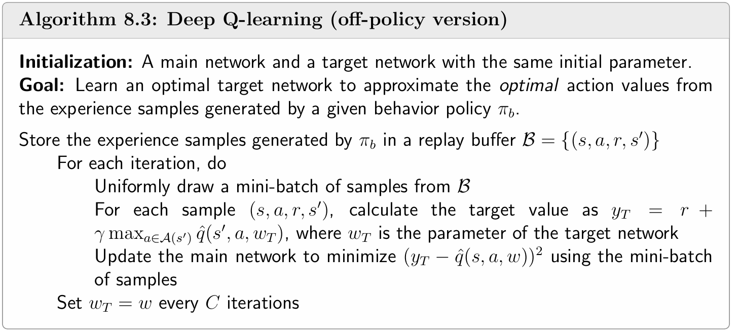

8.4.2 Illustrative examples

This example aims to learn the optimal action values for every state-action pair. Once the optimal action values are obtained, the optimal greedy policy can be obtained immediately.

A single episode is generated by the behavior policy shown in Figure 8.11(a). This behavior policy is exploratory in the sense that it has the same probability of taking any action at any state. The episode has only 1,000 steps as shown in Figure 8.11(b). Although there are only 1,000 steps, almost all the state action pairs are visited in this episode due to the strong exploration ability of the behavior policy. The replay buffer is a set of 1,000 experience samples. The mini-batch size is 100, meaning that we uniformly draw 100 samples from the replay buffer every time we acquire samples.

The main and target networks have the same structure: a neural network with one hidden layer of 100 neurons (the numbers of layers and neurons can be tuned). The neural network has three inputs and one output. The first two inputs are the normalized row and column indexes of a state. The third input is the normalized action index. Here, normalization means converting a value to the interval of $[0,1]$. The output of the network is the estimated action value. The reason why we design the inputs as the row and column of a state rather than a state index is that we know that a state corresponds to a two-dimensional location in the grid. The more information about the state we use when designing the network, the better the network can perform. Moreover, the neural network can also be designed in other ways. For example, it can have two inputs and five outputs, where the two inputs are the normalized row and column of a state and the outputs are the five estimated action values for the input state.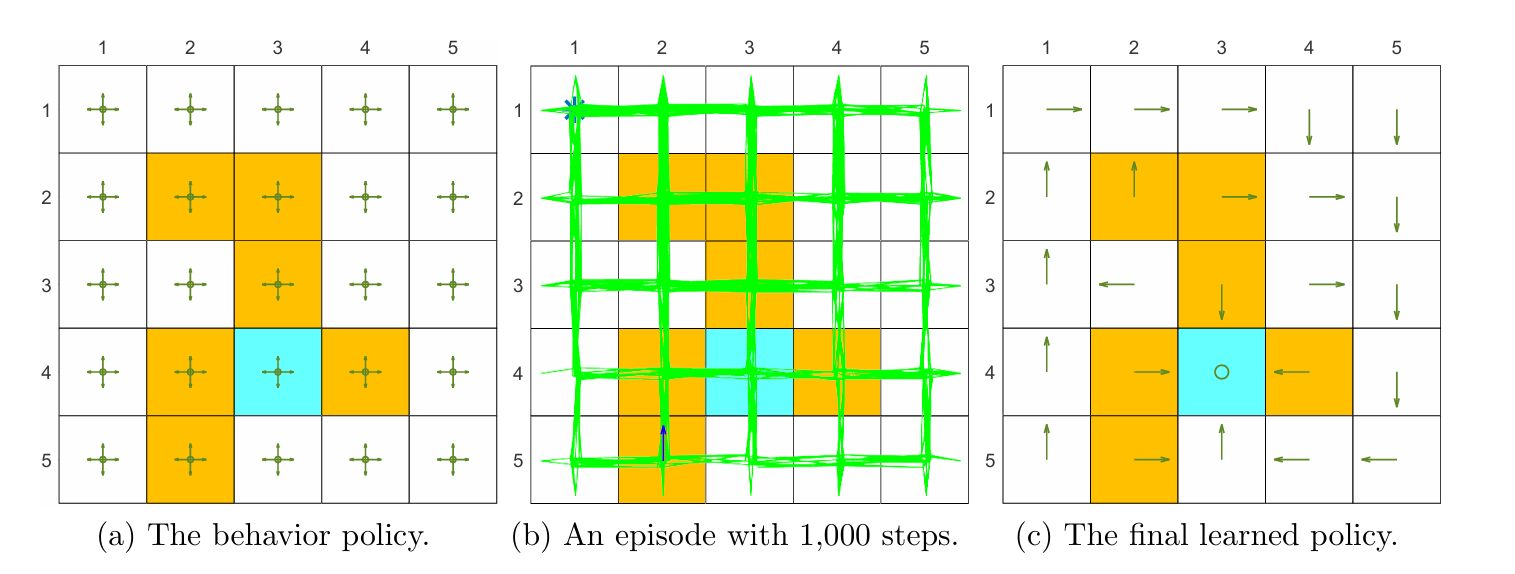

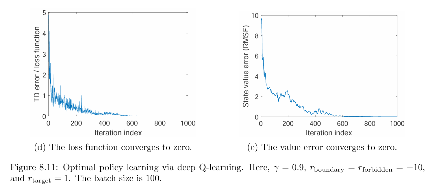
As shown in Figure 8.11(d), the loss function, defined as the average squared TD error of each mini-batch, converges to zero, meaning that the network can fit the training samples well. As shown in Figure 8.11(e), the state value estimation error also converges to zero, indicating that the estimates of the optimal action values become sufficiently accurate. Then, the corresponding greedy policy is optimal.

This example demonstrates the high efficiency of deep Q-learning. In particular, a short episode of 1,000 steps is sufficient for obtaining an optimal policy here. By contrast, an episode with 100,000 steps is required by tabular Q-learning, as shown in Figure 7.4. One reason for the high efficiency is that the function approximation method has a strong generalization ability. Another reason is that the experience samples can be repeatedly used.

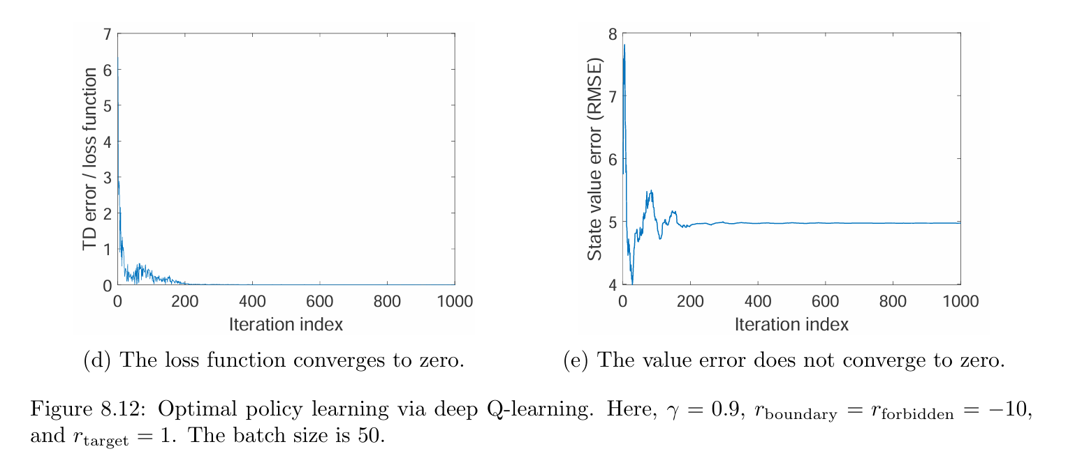
We next deliberately challenge the deep Q-learning algorithm by considering a scenario with fewer experience samples. Figure 8.12 shows an example of an episode with merely 100 steps. In this example, although the network can still be well-trained in the sense that the loss function converges to zero, the state estimation error cannot converge to zero. That means the network can properly fit the given experience samples, but the experience samples are too few to accurately estimate the optimal action values.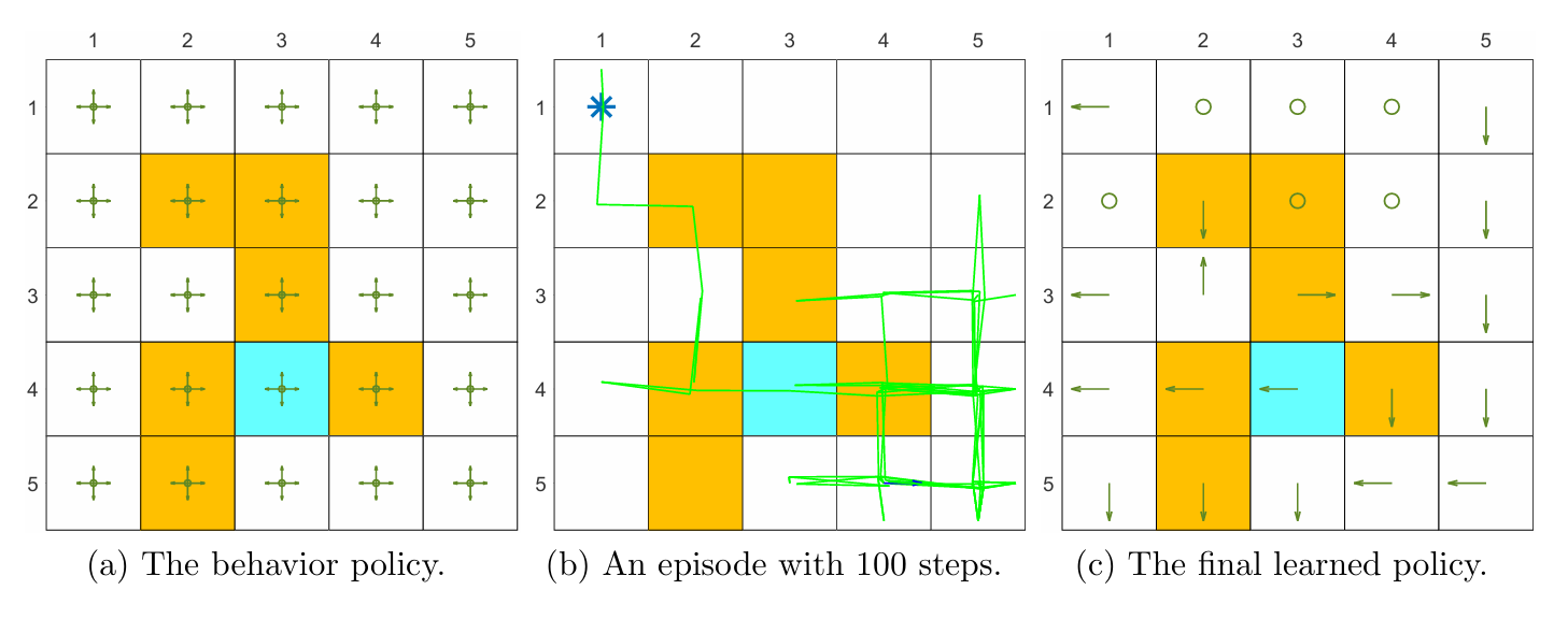

8.5 Summary

This chapter continued introducing TD learning algorithms. However, it switches from the tabular method to the function approximation method. The key to understanding the function approximation method is to know that it is an optimization problem. The simplest objective function is the squared error between the true state values and the estimated values. There are also other objective functions such as the Bellman error and the projected Bellman error. We have shown that the TD-Linear algorithm actually minimizes the projected Bellman error. Several optimization algorithms such as Sarsa and Q-learning with value approximation have been introduced.

One reason why the value function approximation method is important is that it allows artificial neural networks to be integrated with reinforcement learning. For example, deep Q-learning is one of the most successful deep reinforcement learning algorithms.

An important concept named stationary distribution is introduced in this chapter. The stationary distribution plays an important role in defining an appropriate objective function in the value function approximation method. It also plays a key role in Chapter 9 when we use functions to approximate policies. An excellent introduction to this topic can be found in ² .

². M. Pinsky and S. Karlin, An introduction to stochastic modeling Academic Press, 2010.[Chapter IV] ↩

Q: What is the stationary distribution and why is it important?
A: The stationary distribution describes the long-term behavior of a Markov decision process. More specifically, after the agent executes a given policy for a sufficiently long period, the probability of the agent visiting a state can be described by this stationary distribution. More information can be found in Box 8.1.

The reason why this concept emerges in this chapter is that it is necessary for defining a valid objective function. In particular, the objective function involves the probability distribution of the states, which is usually selected as the stationary distribution. The stationary distribution is important not only for the value approximation method but also for the policy gradient method, which will be introduced in Chapter 9.

Q: What are the advantages and disadvantages of the linear function approximation method?
A: Linear function approximation is the simplest case whose theoretical properties can be thoroughly analyzed. However, the approximation ability of this method is limited. It is also nontrivial to select appropriate feature vectors for complex tasks. By contrast, artificial neural networks can be used to approximate values as black-box universal nonlinear approximates, which are more friendly to use. Nevertheless, it is still meaningful to study the linear case to better grasp the idea of the function approximation method. Moreover, the linear case is powerful in the sense that the tabular method can be viewed as a special linear case (Box 8.2).

Q: Can tabular Q-learning use experience replay?
A: Although tabular Q-learning does not require experience replay, it can also use experience relay without encountering problems. That is because Q-learning has no requirements about how the samples are obtained due to its off-policy attribute. One benefit of using experience replay is that the samples can be used repeatedly and hence more efficiently

Approximation (DQN Steps)

Replay buffer

Replay buffer (or experience replay in the original paper) is used in DQN to make the samples i.i.d.

from collections import deque

class ReplayBuffer(object):
    def __init__(self, capacity):
        self.buffer = deque(maxlen=capacity)
    
    def push(self, state, action, reward, next_state, done):
        # print("State shape:", state.shape)
        # print("Next state shape:", next_state.shape)
        
        state      = np.expand_dims(state, 0)
        next_state = np.expand_dims(next_state, 0)
            
        self.buffer.append((state, action, reward, next_state, done))
    
    def sample(self, batch_size):
        state, action, reward, next_state, done = zip(*random.sample(self.buffer, batch_size))
        return np.concatenate(state), action, reward, np.concatenate(next_state), done
    
    def __len__(self):
        return len(self.buffer)

Target network

Firstly, it is possible to build a DQN with a single Q Network and no Target Network. In that case, we do two passes through the Q Network, first to output the Predicted Q value, and then to output the Target Q value.

But that could create a potential problem. The Q Network’s weights get updated at each time step, which improves the prediction of the Predicted Q value. However, since the network and its weights are the same, it also changes the direction of our predicted Target Q values. They do not remain steady but can fluctuate after each update. This is like chasing a moving target.

By employing a second network that doesn’t get trained, we ensure that the Target Q values remain stable, at least for a short period. But those Target Q values are also predictions after all and we do want them to improve, so a compromise is made. After a pre-configured number of time-steps, the learned weights from the Q Network are copied over to the Target Network.

This is like EMA?

DQN

class DQN(nn.Module):
    def __init__(self, num_inputs, num_actions, device='cuda'):
        super(DQN, self).__init__()
        
        self.device = device
        self.num_inputs = num_inputs
        self.num_actions = num_actions
        self.layers = nn.Sequential(
            nn.Linear(num_inputs, 128),
            nn.ReLU(),
            nn.Linear(128, 128),
            nn.ReLU(),
            nn.Linear(128, num_actions)
        ).to(self.device)
        
    def forward(self, x):
        return self.layers(x)
    
    def act(self, state, epsilon):
        if random.random() > epsilon:
            with torch.no_grad():  # Ensures that no gradients are computed, which saves memory and computations
                state = torch.FloatTensor(state).unsqueeze(0).to(self.device)  # Convert state to tensor and add batch dimension
                q_value = self.forward(state)  # Get Q-values for all actions
                action = q_value.max(1)[1].item()  # Get the action with the maximum Q-value and convert to integer
        else:
            action = random.randrange(self.num_actions)
        return action

LOSS

def compute_td_loss(batch_size, replay_buffer, model, gamma, optimizer):
    state, action, reward, next_state, done = replay_buffer.sample(batch_size)

    # Convert numpy arrays to torch tensors
    state = torch.FloatTensor(state).to(model.device)
    next_state = torch.FloatTensor(next_state).to(model.device)
    action = torch.LongTensor(action).to(model.device)
    reward = torch.FloatTensor(reward).to(model.device)
    done = torch.FloatTensor(done).to(model.device)

    # Compute Q-values for current states
    q_values = model(state)

    # Compute Q-values for next states using no gradient computation to speed up and reduce memory usage
    with torch.no_grad():
        next_q_values = model(next_state)
        next_q_value = next_q_values.max(1)[0]  # Get the max Q-value along the action dimension

    # Calculate the expected Q-values
    expected_q_value = reward + gamma * next_q_value * (1 - done)

    # Compute the loss between actual Q values and the expected Q values
    q_value = q_values.gather(1, action.unsqueeze(1)).squeeze(1)
    loss = (q_value - expected_q_value.detach()).pow(2).mean()  # Detach expected_q_value to prevent gradients from flowing

    # Backpropagation
    optimizer.zero_grad()
    loss.backward()
    optimizer.step()

    return loss

Training process

num_frames = 10000
batch_size = 32
gamma      = 0.99

losses = []
all_rewards = []
episode_reward = 0

state, info = env.reset()
for frame_idx in range(1, num_frames + 1):
    epsilon = epsilon_by_frame(frame_idx)
    action = model.act(state, epsilon)
    
    # print(f"Select action: {action}. type: {type(action)}")
    next_state, reward, terminated, truncated, info = env.step(action)
 
    
    replay_buffer.push(state, action, reward, next_state, terminated)
    
    state = next_state
    episode_reward += reward
    
    if terminated:
        state, info = env.reset()
        all_rewards.append(episode_reward)
        episode_reward = 0
        
    if len(replay_buffer) > batch_size:
        loss = compute_td_loss(batch_size, replay_buffer, model, gamma, optimizer)
        losses.append(loss.data.item())
        
        
    if frame_idx % 200 == 0:
        plot(frame_idx, all_rewards, losses)