[toc]
Sources:
9 Policy Gradient Methods
So far in this book, policies have been represented by tables: the action probabilities of all states are stored in a table (e.g., Table 9.1). In this chapter, we show that policies can be represented by parameterized functions denoted as $\pi(a|s,\theta)$, where $\theta \in \mathbb{R}^m$ is a parameter vector. It can also be written in other forms such as $\pi_{\theta}(a|s)$, $\pi_{\theta}(a,s)$, or $\pi(a,s,\theta)$.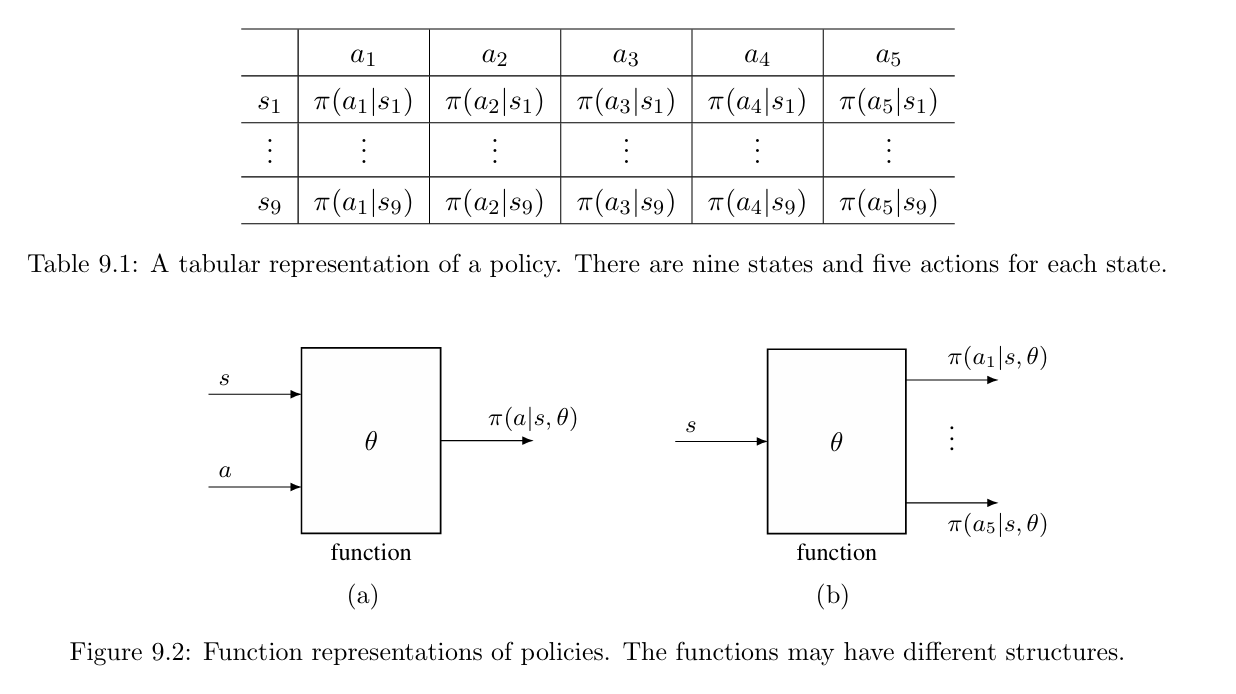
When policies are represented as functions, optimal policies can be obtained by optimizing certain scalar metrics. Such a method is called policy gradient.The policy gradient method is a big step forward in this book because it is policy-based. The advantages of the policy gradient method are numerous. For example, it is more efficient for handling large state/action spaces. It has stronger generalization abilities and hence is more efficient in terms of sample usage.
9.1 Policy representation:From table to function
| Difference | Tabular case | Function representation |
|---|---|---|
| how to define optimal policies? | maximize every state value. | maximize certain scalar metrics. |
| how to update a policy? | directly changing the entries in the table. | changing the parameter $\theta$ |
| how to retrieve the probability of an action? | directly obtained by looking up the table. | input $(s,a)$ or $s$ into the function to calculate its probability(e.g.,Table 9.2) |
The basic idea of the policy gradient method is summarized below. Suppose that $J(\theta)$ is a scalar metric. Optimal policies can be obtained by optimizing this metric via the gradient-based algorithm:
where $\nabla_\theta J$ is the gradient of $J$ with respect to $\theta$ , $t$ is the time step, and $\alpha$ is the optimization rate.
With this basic idea, we will answer the following three questions in the remainder of this chapter.
- What metrics should be used? (Section 9.2).
- How to calculate the gradients of the metrics? (Section 9.3)
- How to use experience samples to calculate the gradients? (Section 9.4)
9.2 Metrics for defining optimal policies
If a policy is represented by a function, there are two types of metrics for defining optimal policies. One is based on state values and the other is based on immediate rewards.
Metric 1: Average state value(Average value)
where $d(s)$ is the weight of state $s$ (probability distribution).It satisfies $d(s)\geq0$ for any $s \in S$ and $\sum_{s \in S}d(s) = 1$.
How to select the distribution $d$ ? There are two cases.
The first and simplest case is that $d$ is independent of the policy $\pi$. In this case, we specifically denote $d$ as $d_0$ and $\bar{v}_{\pi}$ as $\bar{v}_{\pi}^0$ to indicate that the distribution is independent of the policy.
——- One case is to treat all the states equally important and select $d_0(s) = 1/|S|$. (random)
——- Another case is when we are only interested in a specific state $s_0$ (e.g., the agent always starts from $s_0$). In this case, we can design $d_0(s_0)=1, d_0(s \neq s_0)=0 $.The second case is that $d$ is dependent on the policy $\pi$.In this case, it is common to select $d$ as $d_{\pi}$ , which is the stationary distribution under $\pi$.
The interpretation of selecting $d_{\pi}$ is as follows. The stationary distribution reflects the long-term behavior of a Markov decision process under a given policy. If one state is frequently visited in the long term, it is more important and deserves a higher weight; if a state is rarely visited, then its importance is low and deserves a lower weight.
Suppose that an agent collects rewards $\{R_{t+1}\}_{t=0}^\infty$ by following a given policy $\pi(\theta)$. Readers may often see the following metric in the literature(red and blue):
Metric 2: Average reward (Average one-step reward)
where $d_{\pi}$ is the stationary distribution, $r_{\pi}(s)$ is the expectation of the immediate rewards.
Suppose that an agent collects rewards $\{R_{t+1}\}_{t=0}^\infty$ by following a given policy $\pi(\theta)$. A common metric that readers may often see in the literature is
Up to now, we have introduced two types of metrics: $\bar{v}_{\pi}$ and $\bar{r}_{\pi}$ . Each metric has several different but equivalent expressions. They are summarized in Table 9.2.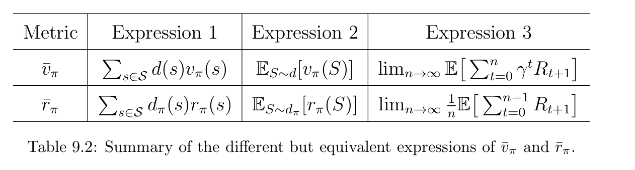
All these metrics are functions of $\pi$. Since $\pi$ is parameterized by $\theta$, these metrics are functions of $\theta$. In other words, different values of $\theta$ can generate different metric values. Therefore, we can search for the optimal values of $\theta$ to maximize these metrics. This is the basic idea of policy gradient methods.
The two metrics $\bar{v}_{\pi}$ and $\bar{r}_{\pi}$ are equivalent in the discounted case where $\gamma< 1$. In particular, it can be shown that
Note that $\bar{v}_{\pi}(\theta) = d_{\pi}^Tv_{\pi}$ and $\bar{r}_{\pi}(\theta) = d_{\pi}^Tr_{\pi}$ , where $v_{\pi}$ and $r_{\pi}$ satisfy the Bellman equation $v_{\pi} = r_{\pi} + \gamma P_{\pi}v_{\pi}$ . Multiplying $d_{\pi}^T$ on both sides of the Bellman equation yields
The above equation indicates that these two metrics can be simultaneously maximized.
9.3 Gradients of the metrics
Given the metrics introduced in the last section, we can use gradient-based methods to maximize them. we first provide the policy gradient theorem(gradent ascent),and then provide the inference process.
Theorem 9.1 (Policy gradient theorem). The gradient of $J(\theta )$ is
where is $\eta$ a state distribution and $\nabla_{\theta}\pi$ is the gradient of $\pi$ with respect to $\theta$. $\ln$ is the natural logarithm. A natural logarithm function is introduced to express the gradient as an expected value $ \nabla_{\theta}\ln A(\theta)=\frac{\nabla_{\theta}A(\theta)}{A(\theta)} $. In this way, we can approximate the true gradient with a stochastic one. It is notable that $\pi(a|s,\theta)$must be positive for all $(s,a)$ to ensure that $\ln\pi(a|s,\theta)$ is valid.This can be achieved by using softmax functions(Relu functions):
Since $\pi(a|s,\theta) > 0$ for all $a$, the parameterized policy is stochastic and hence exploratory.
Theorem 9.1 is a summary of the results in Theorem 9.2, 9.3,and 9.5. These three theorems address different scenarios involving different metrics and discounted/undiscounted cases, but the gradients in these scenarios all have similar expressions. In particular, $J(\theta)$ could be $\bar{v}_{\pi}^0$, $\bar{v}_{\pi}$, or $\bar{r}_{\pi}$. The equality in Theorem 9.1 may become a strict equality or an approximation. The distribution also varies in different scenarios.
- distinguish different metrics $\bar{v}_{\pi}^0$, $\bar{v}_{\pi}$, or $\bar{r}_{\pi}$
- distinguish the discounted and undiscounted cases.
9.3.1 Derivation of the gradients in the discounted case
Theorem 9.2 (Gradient of $\bar{v}_{\pi}^0$ in the discounted case). In the discounted case where $\gamma \in (0,1)$, the gradient of $\bar{v}_{\pi}^0= d_0^Tv_{\pi}$ is
Theorem 9.3 (Gradients of $\bar{r}_{\pi}$ and $\bar{v}_{\pi}$ in the discounted case). In the discounted case where $\gamma \in (0,1)$, the gradients of $\bar{r}_{\pi}$ and $\bar{v}_{\pi}$ are
Here, the approximation is more accurate when $\gamma$ is closer to 1.
9.3.2 Derivation of the gradients in the undiscounted case
the undiscounted case means $ \gamma = 1$. Why we suddenly start considering the undiscounted case,The reasons are as follows. First, for continuing tasks, it may be inappropriate to introduce the discount rate and we need to consider the undiscounted case. Second, While the gradient of $\bar{r}_{\pi}$ in the discounted case is an approximation, we will see that its gradient in the undiscounted case is more elegant.
Theorem 9.3 (Gradient of $\bar{r}_{\pi}$ in the undiscounted case). In the undiscounted case, the gradient of the average reward $\bar{r}_{\pi}$ is
| metric | derivative of the metric | ||
|---|---|---|---|
| general case$J(\theta)$ | $ \nabla_{\theta}J(\theta)=\sum \eta(s)\sum\nabla_{\theta}\pi(a\ | s,\theta)q_{\pi}(s,a)=E(\nabla ln \pi(a\ | s,\theta)q_{\pi}(s,a)) $ |
| $\bar v_{\pi}^0=d_0^Tv_{\pi}$ | $ \nabla_{\theta} \bar v_{\pi}^0=\sum d_0(s^{‘})[(I-\gamma P_{\pi})^{-1}]_{s’s}\sum \pi(a\ | s,\theta)\nabla_{\theta}ln{\pi}(a\ | s,\theta)q_{\pi}(s,a) $ |
| $\bar v_{\pi}=d_{\pi}^T \bar v_{\pi}$ | $ \nabla_{\theta} \bar v_{\pi}=(1-\gamma)^{-1} \sum d_{\pi}(s)\sum \nabla_{\theta}\pi (a\ | s,\theta)q_{\pi}(s,a) $ | |
| $\bar r_{\pi}=d_{\pi}^T \bar r_{\pi}$ | $ \nabla_{\theta} \bar r_{\pi}= (1-\gamma) \nabla_{\theta} \bar v_{\pi} $ |
9.4 Monte Carlo policy gradient (REINFORCE)
The gradient-ascent algorithm for maximizing $J(\theta)$ is
where $q_t(s_t, a_t)$ is an approximation of $q_{\pi}(s_t, a_t)$. If $qt(st at)$ is obtained by Monte Carlo estimation, the algorithm is called REINFORCE 1 or Monte Carlo policy gradient, which is one of earliest and simplest policy gradient algorithms.
REINFORCE is important since many other policy gradient algorithms can be obtained by extending it.
We next examine the interpretation of (11) more closely. Since $\nabla_{\theta}\ln\pi(a_t|s_t,\theta_t)=\frac{\nabla_{\theta}\pi(a_t|s_t,\theta_t)}{\pi(a_t|s_t,\theta_t)}$ , we can rewrite (11) as
Two important interpretations can be seen from this equation.
If $\beta_t \geq 0$,the probability of choosing $(s_t,a_t)$ is enhanced. $\pi(a_t|s_t,\theta_{t+1})\geq \pi(a_t|s_t,\theta_{t})$, The greater $\beta_t$ is, the stronger the enhancement is.
If $\beta_t \leq 0$,the probability of choosing $(s_t,a_t)$ decreases. $\pi(a_t|s_t,\theta_{t+1})\leq \pi(a_t|s_t,\theta_{t})$.The algorithm can strike a balance between exploration and exploitation.
$\beta_t$ is proportional to $q_t(s_t,a_t)$. If the action value of $(s_t,a_t)$ is large, then $\theta_{t+1}$ is change to make $\pi(a_t|s_t,\theta_t)$ enhance so that the probability of selecting at $a_t$ increases. Therefore, the algorithm attempts to exploit actions with greater values.
$\beta_t$ is inversely proportional to $\pi(a_t|s_t,\theta_t)$ when $q_t(s_t,a_t)>0$. As a result, if the probability of selecting $a_t$ is small, then $\beta_t$ is enhanced so that $\theta_{t+1}$ make the probability of selecting $a_t$ increases ($\pi(a_t|s_t,\theta_t)$). Therefore, the algorithm attempts to explore actions with low probabilities.
Moreover, since (12) uses samples to approximate the true gradient, it is important to understand how the samples should be obtained.
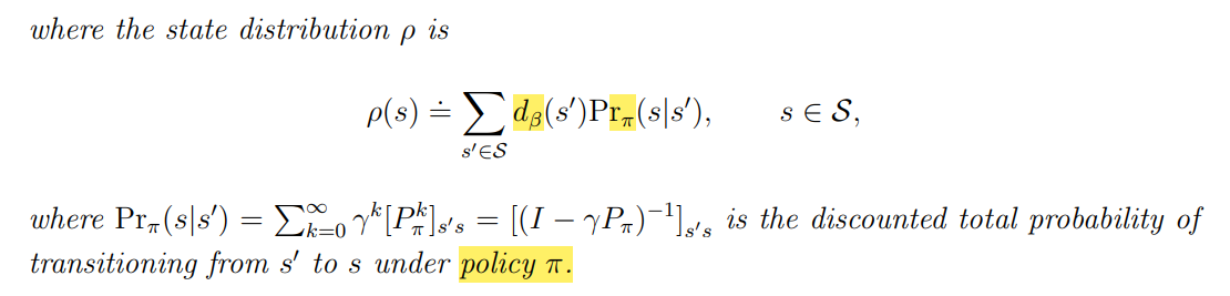
How to sample $S$? $S$ in the true gradient $\mathbb{E}[\nabla_\theta \ln\pi(A|S, \theta_t)q_{\pi}(S,A)]$ should obey the distribution $\eta$ which is either the stationary distribution $d_{\pi}$ or the discounted total probability distribution $\rho_{\pi}$ in (9). Either $d_{\pi}$ or $\rho_{\pi}$ represents the long-term behavior exhibited under $\pi$.
How to sample $A$? $A$ in $\mathbb{E}[\nabla_\theta \ln\pi(A|S, \theta_t)q_{\pi}(S,A)]$ should obey the distribution of $\pi(A|S,\theta)$. The ideal way to sample $A$ is to select at following $\pi(a|s_t, \theta_t)$. Therefore, the policy gradient algorithm is on-policy.
Unfortunately, the ideal ways for sampling $S$ and $A$ are not strictly followed in practice due to their low efficiency of sample usage.A more sample-efficient implementation of (12) is given in Algorithm 9.1. In this implementation, an episode is first generated by following $\pi(\theta)$. Then, $\theta$ is updated multiple times using every experience sample in the episode.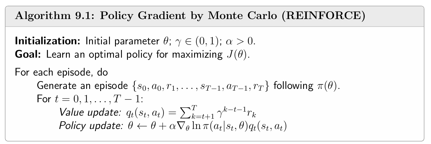 (图片有笔误,计算动作值时从后往前计算$t=T-1,T-2,…,1,0$)
1:R. J. Williams, Simple statistical gradient-following algorithms for connectionist reinforcement learning, Machine Learning, vol. 8, no. 3, pp. 229256, 1992.
9.5 Summary
This chapter introduced the policy gradient method, which is the foundation of many modern reinforcement learning algorithms. Policy gradient methods are policy-based.The basic idea of the policy gradient method is simple. That is to select an appropriate scalar metric and then optimize it via a gradient-ascent algorithm.
The most complicated part of the policy gradient method is the derivation of the gradients of the metrics. That is because we have to distinguish various scenarios with different metrics and discounted/undiscounted cases. Fortunately, the expressions of the gradients in different scenarios are similar.Hence, we summarized the expressions in Theorem 9.1, which is the most important theoretical result in this chapter.
The policy gradient algorithm in (12) must be properly understood since it is the foundation of many advanced policy gradient algorithms. In the next chapter, this algorithm will be extended to another important policy gradient method called actor-critic.
10 Actor-Critic Methods
“actor-critic” refers to a structure that incorporates both policy-based and value-based methods. An actor refers to a policy update step. The reason that it is called an actor is that the actions are taken by following the policy. Here, an critic refers to a value update step. It is called a critic because it criticizes the actor by evaluating its corresponding values. In addition, actor-critic methods are still policy gradient algorithms.
10.1 The simplest actor-critic algorithm (QAC)
The optimal algorithm used by QAC is the same as Section 9.4 Monte Carlo policy gradient (REINFORCE)
The gradient-ascent algorithm for maximizing $J(\theta)$ is
On the one hand, it is a policy-based algorithm since it directly updates the policy parameter ($\theta$). On the other hand, this equation requires knowing $q_t(s_t, a_t)$, which is an estimate of the action value $q_t(s_t, a_t)$. As a result, another value-based algorithm is required to generate $q_t(s_t, a_t)$ (used Monte Carlo learning and temporal-difference (TD) learning).
- If $q_t(s_t, a_t)$ is estimated by Monte Carlo learning, the corresponding algorithm is called REINFORCE or Monte Carlo policy gradient.
- If $q_t(s_t, a_t)$ is estimated by TD learning, the corresponding algorithms are usually called actor-critic. Therefore, actor-critic methods can be obtained by incorporating TD-based value estimation into policy gradient methods.
The procedure of the simplest actor-critic algorithm is summarized in Algorithm 10.1.This actor-citric algorithm is sometimes called Q actor-critic (QAC). Although it is simple, QAC reveals the core idea of actor-critic methods.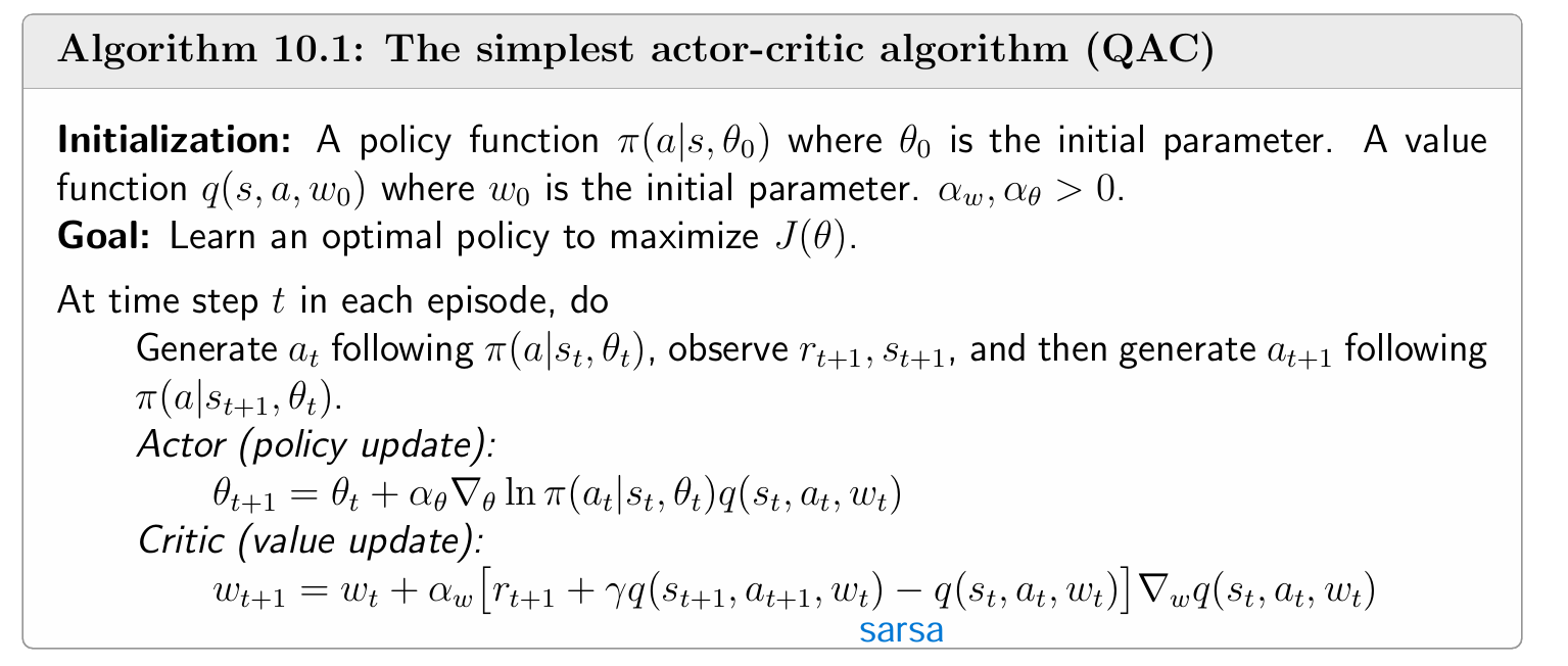
10.2 Advantage actor-critic (A2C)
The core idea of A2C is to introduce a baseline to reduce estimation variance.
A2C算法可以看作是传统PG算法的一种扩展,引入了value-based方法。当我们采用一个函数来近似动作值并利用TD算法(随机梯度下降)来拟合该函数时,该方法被称为QAC算法。
在实际应用中,REINFORCE和QAC由于估计的方差较大,因此效果并不好。A2C算法通过在’动作值‘的估计中引入偏置量来降低SGD中对于梯度估计的方差,近似最优偏置量为状态值$v_{\pi}(s_t)$
10.2.1 Baseline invariance
One interesting property of the policy gradient is that it is invariant to an additional baseline.
where the additional baseline $b(S)$ is a scalar function of $S$. Note:The bias of $b(S)$ should only be related to the environment, because if it is related to the interaction strategy $\pi$, $b(S)$ will change with the change of strategy.
Equation (10.3) holds if and only if:
why is the baseline useful?
The baseline is useful because it can reduce the approximation variance when we use samples to approximate the true gradient.
We need to use a stochastic sample $x(s,a)$ to approximate $E[X(S,A)]$, According to equation 10.1, $E[X(S,A)]$ is invariant to the baseline, but the variance $var(X)$ is not. Our goal is to design a good baseline to minimize $var(X)$. In the algorithms of REINFORCE and QAC, we set $b=0$, which is not guaranteed to be a good baseline.
In fact, the optimal baseline that minimizes $var(X)$ is (proof by BOX10.1)
Although the baseline in(10.5) is optimal, it is too complex to be useful in practice. If the weight $||\nabla_{\theta}\ln\pi(A|s,\theta_t)||^2$ is removed from (10.5), we can obtain a suboptimal
baseline that has a concise expression:
Interestingly, this suboptimal baseline is the state value.
10.2.2 Algorithm description
When $b(s) = v_{\pi} (s)$, the gradient-ascent algorithm in (10.1) becomes
More specifically, note that $v_{\pi}(s) = \sum_{a \in A} \pi(a|s)q_{\pi}(s,a)$ is the mean of the action values. If $\delta_{\pi}(s,a) > 0$, it means that the corresponding action has a greater value than the mean value.
Here, $q_t(s_t, a_t)$ and $v_t(s_t)$ are approximations of $q_{\pi(\theta_t)}(s_t,a_t)$ and $v_{\pi(\theta_t)}(s_t)$, respectively. The algorithm in (10.7) updates the policy based on the relative value of $q_t$ with respect to $v_t$ rather than the absolute value of $q_t$. This is intuitively reasonable because, when we attempt to select an action at a state, we only care about which action has the greatest value relative to the others.
If $q_t(s_t, a_t)$ and $v_t(s_t)$ are estimated by Monte Carlo learning, the algorithm in (10.7) is called REINFORCE with a baseline. If $q_t(s_t, a_t)$ and $v_t(s_t)$ are estimated by TD learning, the algorithm is usually called advantage actor-critic (A2C). The implementation of A2C is summarized in Algorithm 10.2.
the advantage function in this implementation is approximated by the TD error:
One merit of using the TD error is that we only need to use a single neural network to represent $v_{\pi} (s)$. Otherwise, we need to maintain two networks to represent $q_{\pi}(s, a)$ and $v_{\pi}(s)$, respectively. The algorithm may also be called TD actor critic. In addition, it is notable that the policy $\pi(\theta_t)$ is stochastic and hence exploratory. Therefore, it can be directly used to generate experience samples without relying on techniques such as $\epsilon$-greedy. There are some variants of A2C such as asynchronous advantage actor-critic (A3C). Interested readers may check 23.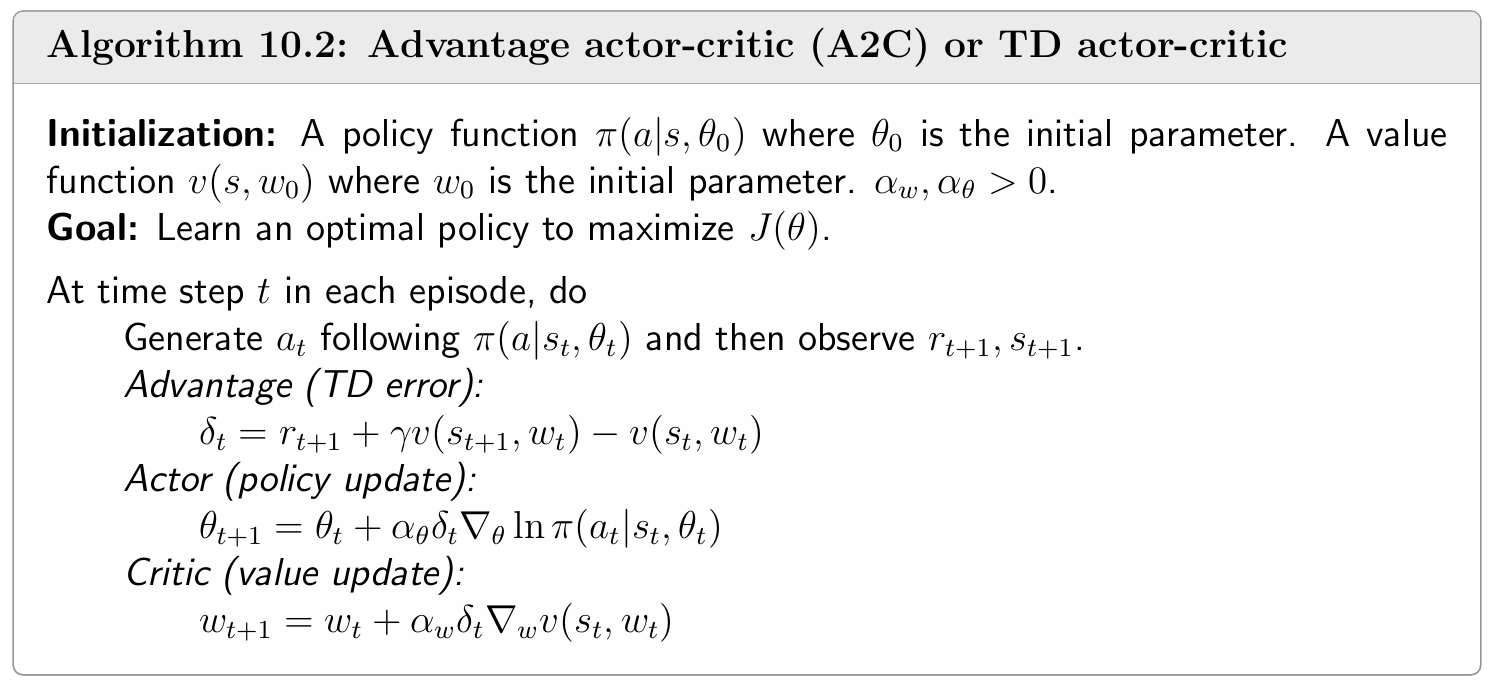
2. V. Mnih, A. P. Badia, M. Mirza, A. Graves, T. Lillicrap, T. Harley, D. Silver, and K. Kavukcuoglu, Asynchronous methods for deep reinforcement learning, in International Conference on Machine Learning, pp. 19281937, 2016. ↩
3. M. Babaeizadeh, I. Frosio, S. Tyree, J. Clemons, and J. Kautz, Reinforcement learning through asynchronous advantage actor-critic on a GPU, arXiv:1611.06256, 2016. ↩
10.3 Off-policy actor-critic
we can employ a technique called importance sampling. It is worth mentioning that the importance sampling technique is not restricted to the field of reinforcement learning. It is a general technique for estimating expected values defined over one probability distribution using some samples drawn from another distribution.
The advantage of off-policy compared to on-policy is that it can ensure that the converged policy in a stata will not diverge again, and the convergence is guaranteed. However, there will be a loss in exploration, which is inevitable.
_Question:off-policy actor-critic算法的优点是什么?为什么要提出off-policy算法?(Hint:强化学习要解决的本质问题是exploration-exploitation)
注:在实践中,由于Off-Policy Actor-Critic算法中actor和critic参数更新的步长中含有
因此当采样策略与优化策略差距过大时(尤其当因此当采样策略与优化策略差距过大时(尤其当$\pi(\theta)与\beta$差异较大时,参数更新公式中的重要性因子会导致梯度爆炸),算法效果不佳(可以考虑PPO对优化目标添加正则项裁切梯度,或考虑DPG避免对动作值进行直接采样)
10.3.1 Importance sampling
$\frac{p_0(x)}{p_1(x)}$ is called the importance weight(it need be set). When $p_1 = p_0$, the importance weight is 1 and $\bar{f}$ becomes $\bar{x}$. When $p_0(x_i) ≥ p_1(x_i)$, $x_i$ can be sampled more frequently by $p_0$ but less frequently by $p_1$. In this case, the importance weight, which is greater than one, emphasizes the importance of this sample. $p_0$ is target policy, $p_1$ is behaviors policy
The importance weight can be understood as follows: the samples corresponding to $p_0$ being large but $p_1$being small are more important, while the samples corresponding to $p_0$ being small but $p_1$ being large become less important.
10.3.2 The off-policy policy gradient theorem
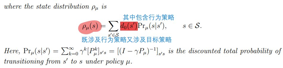
With the importance sampling technique, we are ready to present the off-policy policy gradient theorem. Suppose that $\beta$ is a behavior policy. Our goal is to use the samples generated by $\beta$ to learn a target policy $\pi$ that can maximize the following metric:
The gradient is similar to that in the on-policy case in Theorem 9.1, but there are two differences. The first difference is the importance weight. The second difference is that $A ∼ β$ instead of $A ∼ π$.
10.3.3 Algorithm description
Because $\mathbb{E}\left[\frac{\pi(A | S,\theta)}{\beta(A | S)} \nabla_{\theta}\ln\pi(A|S,\theta_t)b(S)\right] = 0$ To reduce the estimation variance, we can select the baseline as $b(S) = v_{\pi}(S)$ and obtain
Importance weight is included in both the critic and the actor.
It must be noted that, in addition to the actor, the critic is also converted from on-policy to off-policy by the importance sampling technique. In fact, importance sampling is a general technique that can be applied to both policy-based and value-based algorithms. Finally, Algorithm 10.3 can be extended in various ways to incorporate more techniques such as eligibility traces 4.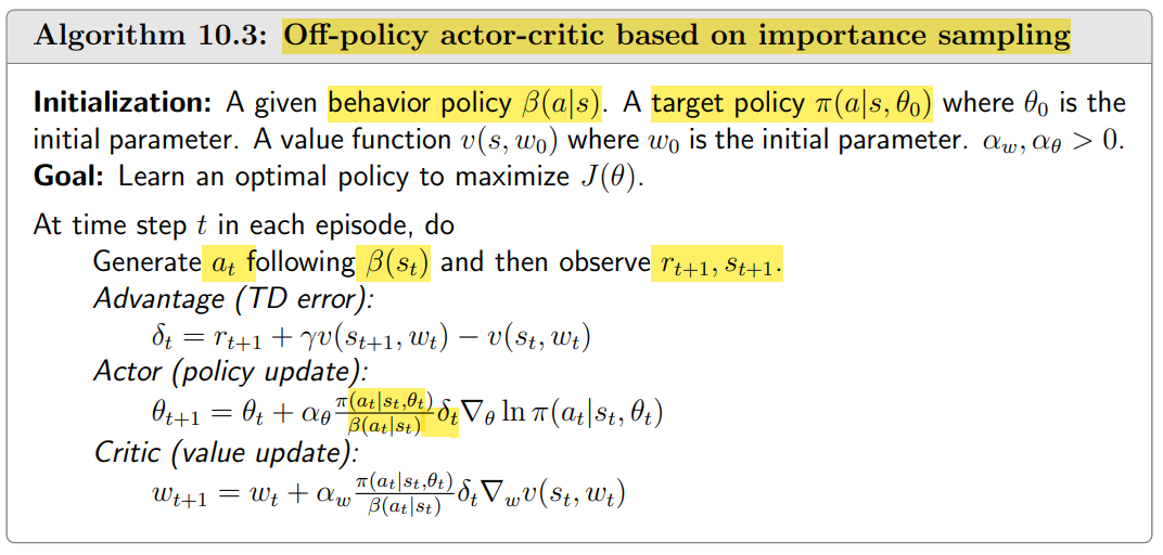
4:T. Degris, M. White, and R. S. Sutton, “Off-policy actor-critic,” arXiv:1205.4839,2012.
10.4 Deterministic actor-critic
Up to now, the policies used in the policy gradient methods are all stochastic since it is required that $\pi(a|s, \theta) > 0$ for every $(s, a)$. This section shows that deterministic policies can also be used in policy gradient methods. Here, “deterministic” indicates that, for any state, a single action is given a probability of one and all the other actions are given probabilities of zero. It is important to study the deterministic case since it is naturally off-policy and can effectively handle continuous action spaces and large scale action spaces.
We have been using $\pi(a|s, \theta)$ to denote a general policy, which can be either stochastic or deterministic. In this section, we use to specifically denote a deterministic policy. Different from $\pi$ which gives the probability of an action, $\mu$ directly gives the action since it is a mapping from $\mathbf{S}$ to $\mathbf{A}$. This deterministic policy can be represented by, for example, a neural network with $s$ as its input, $a$ as its output, and $\theta$ as its parameter. For the sake of simplicity, we often write $\mu(s, \theta)$ as $\mu(s)$ for short.
10.4.1 The deterministic policy gradient theorem
The policy gradient theorem introduced in the last chapter is only valid for stochastic policies. When we require the policy to be deterministic, a new policy gradient theorem must be derived.
Theorem 10.2 (Deterministic policy gradient theorem). The gradient of $J(\theta)$ is
where $\eta$ is a distribution of the states.
Unlike the stochastic case, the gradient in the deterministic case shown in (10.9) does not involve the action random variable $A$ (because $a=\mu(S)$). As a result, when we use samples to approximate the true gradient, it is not required to sample actions. Therefore, the deterministic policy gradient method is off-policy.
Theorem 10.3 (Deterministic policy gradient theorem in the discounted case). in the discounted case where $γ ∈ (0, 1)$, the gradient of $J(θ)$ is
Theorem 10.4 (Deterministic policy gradient theorem in the undiscounted case). In the undiscounted case, the gradient of $J(θ)$ is
where $d_{\mu}$ is the stationary distribution of the states under policy $\mu$.
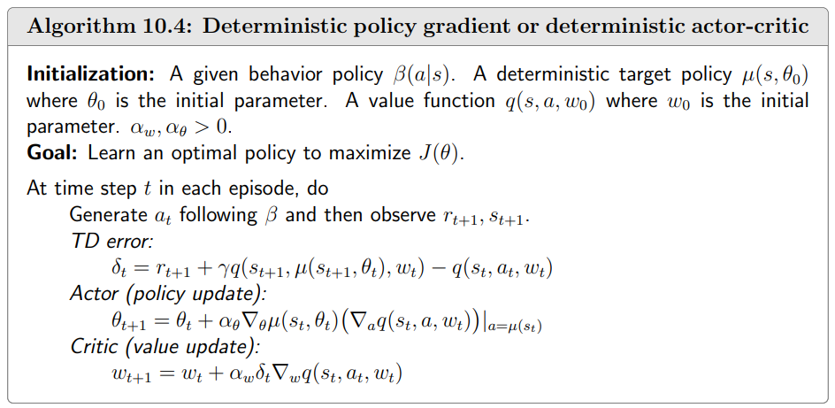
10.4.2 Algorithm description
It should be noted that this algorithm is off-policy since the behavior policy $β$ may be different from $µ$. First, the actor is off-policy. We already explained the reason when presenting Theorem 10.2.
Second, the critic is also off-policy. Special attention must be paid to why the critic is off-policy but does not require the importance sampling technique. In particular, the experience sample required by the critic is $(s_t, a_t, r_{t+1}, s_{t+1}, \textcolor{red}{\tilde{a}_{t+1}})$, where $\tilde{a}_{t+1} = µ(s_{t+1})$. The generation of this experience sample involves two policies. The first is the policy for generating $a_t$ at $s_t$, and the second is the policy for generating $\tilde{a}_{t+1}$ at $s_{t+1}$. The first policy that generates $a_t$ is the behavior policy since $a_t$ is used to interact with the environment. The second policy must be $µ$ because it is the policy that the critic aims to evaluate. Hence, $µ$ is the target policy. It should be noted that $\tilde{a}_{t+1}$ is not used to interact with the environment in the next time step. Hence, $µ$ is not the behavior policy. Therefore, the critic is off-policy.
How to select the function $q(s, a, w)$? The original research work 5 that proposed the deterministic policy gradient method adopted linear functions: $q(s, a, w) = φT(s, a)w$ where $φ(s, a)$ is the feature vector. It is currently popular to represent $q(s, a, w)$ using neural networks, as suggested in the deep deterministic policy gradient (DDPG) method6.
How to select the behavior policy $β$? It can be any exploratory policy. It can also be a stochastic policy obtained by adding noise to $µ$ 6. In this case, $µ$ is also the behavior policy and hence this way is an on-policy implementation.
5. D. Silver, G. Lever, N. Heess, T. Degris, D. Wierstra, and M. Riedmiller, “Deterministic policy gradient algorithms,” in International Conference on Machine Learning, pp. 387–395, 2014. ↩
6. T. P. Lillicrap, J. J. Hunt, A. Pritzel, N. Heess, T. Erez, Y. Tassa, D. Silver, and D. Wierstra, “Continuous control with deep reinforcement learning,” arXiv:1509.02971, 2015. ↩
DPG算法优点:
- 能够处理具有无限元素的动作集合,提高算法的泛化性与训练效率
由于无需直接对动作进行采样,因此是off-policy算法,同时能够避免重要性因子过大导致的梯度爆炸(不恰当的采样策略会导致其与目标策略之间的分布间差异过大)
原因:DPG算法利用梯度上升优化的目标函数表达式为:
可以观察到真实梯度中并不包含对动作值的采样(取而代之的是由Actor Net直接输出的动作值估计),因此是off-policy算法
Question:DPG在数学意义上解决什么问题?与前述stochastic policy gradient算法的critic求解的数学问题有什么不同?(Hint:观察TD Error)
注:考虑到DPG中Actor的输出为动作本身,因此选择gym提供的具有连续动作空间的Pendulum环境进行测试
思考:
- On-policy和Off-policy分别适用于解决什么类型的任务?为什么?
答:On-policy适合解决给定起始状态和终点状态之间最优‘路径’一类问题,Off-policy适合求解任意状态的最优策略。这是由于On-policy算法的behavior policy和target policy是同一个,因此无法保证充分地探索每一个‘状态-动作’对;而Off-policy算法的前述两类policy并非同一个,因此可以选择随机性较强的behavior policy(例如均匀随机策略)来充分探索。- Online和Offline算法分别适用于解决什么类型的任务?为什么?答:Online算法适合样本量较少情况下的学习任务,诸多算法都利用了Generalized Policy Iteration的思想,效率较高;Offline算法适合已经拥有大量样本的情况,因为利用模拟仿真的方法(例如,Monte-Carlo)采样效率较低。
10.5 Summary
In this chapter, we introduced actor-critic methods. The contents are summarized as follows.
Section 10.1 introduced the simplest actor-critic algorithm called QAC. This algorithm is similar to the policy gradient algorithm, REINFORCE, introduced in the last chapter. The only difference is that the q-value estimation in QAC relies on TD learning while REINFORCE relies on Monte Carlo estimation.
Section 10.2 extended QAC to advantage actor-critic. It was shown that the policy gradient is invariant to any additional baseline. It was then shown that an optimal baseline could help reduce the estimation variance.
Section 10.3 further extended the advantage actor-critic algorithm to the off-policy case. To do that, we introduced an important technique called importance sampling.
Finally, while all the previously presented policy gradient algorithms rely on stochastic policies, we showed in Section 10.4 that the policy can be forced to be deterministic. The corresponding gradient was derived, and the deterministic policy gradient algorithm was introduced.
Policy gradient and actor-critic methods are widely used in modern reinforcement learning. There exist a large number of advanced algorithms in the literature such as SAC 7 8, TRPO 9, PPO 10, and TD3 11. In addition, the single-agent case can also be extended to the case of multi-agent reinforcement learning 12 13 14 15 16. Experience samples can also be used to fit system models to achieve model-based reinforcement learning 17 18 19. Distributional reinforcement learning provides a fundamentally different perspective from the conventional one 20 21. The relationships between reinforcement learning and control theory have been discussed in 22 23 24 25 26 27. This book is not able to cover all these topics. Hopefully, the foundations laid by this book can help readers better study them in the future.
7. T. Haarnoja, A. Zhou, P. Abbeel, and S. Levine, “Soft actor-critic: Off-policy maximum entropy deep reinforcement learning with a stochastic actor,” in International Conference on Machine Learning, pp. 1861–1870, 2018. ↩
8. T. Haarnoja, A. Zhou, K. Hartikainen, G. Tucker, S. Ha, J. Tan, V. Kumar, H. Zhu, A. Gupta, and P. Abbeel, “Soft actor-critic algorithms and applications,” arXiv:1812.05905, 2018. ↩
9. J. Schulman, S. Levine, P. Abbeel, M. Jordan, and P. Moritz, “Trust region policy optimization,” in International Conference on Machine Learning, pp. 1889–1897, 2015. ↩
10. J. Schulman, F. Wolski, P. Dhariwal, A. Radford, and O. Klimov, “Proximal policy optimization algorithms,” arXiv:1707.06347, 2017. ↩
11. S. Fujimoto, H. Hoof, and D. Meger, “Addressing function approximation error in actor-critic methods,” in International Conference on Machine Learning, pp. 1587–1596, 2018. ↩
12. J. Foerster, G. Farquhar, T. Afouras, N. Nardelli, and S. Whiteson, “Counterfactual multi-agent policy gradients,” in AAAI Conference on Artificial Intelligence,vol. 32, 2018 ↩
13. R. Lowe, Y. I. Wu, A. Tamar, J. Harb, O. Pieter Abbeel, and I. Mordatch, “Multiagent actor-critic for mixed cooperative-competitive environments,” Advances in Neural Information Processing Systems, vol. 30, 2017. ↩
14. Y. Yang, R. Luo, M. Li, M. Zhou, W. Zhang, and J. Wang, “Mean field multiagent reinforcement learning,” in International Conference on Machine Learning, pp. 5571–5580, 2018. ↩
15. O. Vinyals, I. Babuschkin, W. M. Czarnecki, M. Mathieu, A. Dudzik, J. Chung, D. H. Choi, R. Powell, T. Ewalds, P. Georgiev, et al., “Grandmaster level in StarCraft II using multi-agent reinforcement learning,” Nature, vol. 575, no. 7782, pp. 350–354, 2019. ↩
16. Y. Yang and J. Wang, “An overview of multi-agent reinforcement learning from game theoretical perspective,” arXiv:2011.00583, 2020. ↩
17. F.-M. Luo, T. Xu, H. Lai, X.-H. Chen, W. Zhang, and Y. Yu, “A survey on modelbased reinforcement learning,” arXiv:2206.09328, 2022. ↩
18. S. Levine and V. Koltun, “Guided policy search,” in International Conference on Machine Learning, pp. 1–9, 2013. ↩
19. M. Janner, J. Fu, M. Zhang, and S. Levine, “When to trust your model: Modelbased policy optimization,” Advances in Neural Information Processing Systems, vol. 32, 2019 ↩
20. M. G. Bellemare, W. Dabney, and R. Munos, “A distributional perspective on reinforcement learning,” in International Conference on Machine Learning, pp. 449–458, 2017. ↩
21. M. G. Bellemare, W. Dabney, and M. Rowland, Distributional Reinforcement Learning. MIT Press, 2023 ↩
22. H. Zhang, D. Liu, Y. Luo, and D. Wang, Adaptive dynamic programming for control:algorithms and stability. Springer Science & Business Media, 2012. ↩
23. F. L. Lewis, D. Vrabie, and K. G. Vamvoudakis, “Reinforcement learning and feedback control: Using natural decision methods to design optimal adaptive controllers,” IEEE Control Systems Magazine, vol. 32, no. 6, pp. 76–105, 2012. ↩
24. F. L. Lewis and D. Liu, Reinforcement learning and approximate dynamic programming for feedback control. John Wiley&Sons, 2013. ↩
25. Z.-P. Jiang, T. Bian, and W. Gao, “Learning-based control: A tutorial and some recent results,” Foundations and Trends in Systems and Control, vol. 8, no. 3, pp. 176–284, 2020. ↩
26. S. Meyn, Control systems and reinforcement learning. Cambridge University Press, 2022. ↩
27. S. E. Li, Reinforcement learning for sequential decision and optimal control. Springer, 2023. ↩