Mathematical Foundation of Reinforcement Learning - Algorithms (model-based & non-incremental)

[toc]

Reference Sources:

1. Shiyu Zhao. 《Mathematical Foundation of Reinforcement Learning》Chapter 4-5.
2. OpenAI Spinning Up
3. Lu yukuan’s notes

4. Value iteration and policy iteration(dynamic programming algorithms)

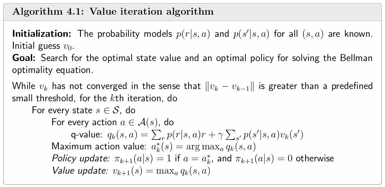
4.1 Value iteration

The value iteration algorithm is exactly the algorithm suggested by the contraction mapping theorem for solving the Bellman optimality equation (BOE).

The BOE Solution algorithm is

$$\begin{equation} v_{k+1}=\max _{\pi \in \Pi}\left(r_\pi+\gamma P_\pi v_k\right), \quad k=0,1,2, \ldots \end{equation}$$

It is guaranteed that $v_k$ and $\pi_k$ converge to the optimal state value and an optimal policy as $k \rightarrow \infty$, respectively.

value iteration is an iterative algorithm. Each iteration has two steps.
Step 1: policy update($v_k$ → $\pi_{k+1}$). This step is to solve

$$\begin{equation} \pi_{k+1}=\arg \max _\pi\left(r_\pi+\gamma P_\pi v_k\right) \end{equation}$$

where $v_k$ is obtained in the previous iteration.$v_0$ can be random setting.

Step 2: value update($v_k$,$\pi_{k+1}$ → $v_{k+1}$).

$$\begin{equation} v_{k+1}=r_{\pi_{k+1}}+\gamma P_{\pi_{k+1}} v_k, \end{equation}$$

where $v_{k+1}$ will be used in the next iteration.

The value iteration algorithm introduced above is in a matrix-vector form. It’s useful for understanding the core idea of the algorithm. To implement this algorithm, we need to further examine its elementwise form.

---

Step 1: Policy update(elementwise form)

The elementwise form of $\pi_{k+1}$ is

$$\pi_{k+1}(s)=\arg \max _\pi \sum_a \pi(a \mid s) \underbrace{\left(\sum_r p(r \mid s, a) r+\gamma \sum_{s^{\prime}} p\left(s^{\prime} \mid s, a\right) v_k\left(s^{\prime}\right)\right)}_{q_k(s, a)}, \quad s \in \mathcal{S}$$

The optimal policy solving the above optimization problem is

$$\pi_{k+1}(a \mid s)=\left\{\begin{array}{cc} 1 & a=a_k^*(s) \\ 0 & a \neq a_k^*(s) \end{array}\right.$$

where $a_k^(s)=\arg \max _a q_k(a, s).
\pi_{k+1}$ is called a *greedy policy, since it simply selects the greatest q-value.

Step 2: Value update(elementwise form)

The elementwise form of $v_{k+1}$ is

$$v_{k+1}(s)=\sum_a \pi_{k+1}(a \mid s) \underbrace{\left(\sum_r p(r \mid s, a) r+\gamma \sum_{s^{\prime}} p\left(s^{\prime} \mid s, a\right) v_k\left(s^{\prime}\right)\right)}_{q_k(s, a)}, \quad s \in \mathcal{S}$$

Since $\pi_{k+1}$ is greedy, the above equation is simply

$$v_{k+1}(s)=\max _a q_k(a, s)$$

Procedure summary:

$v_k(s) \rightarrow q_k(s, a) \rightarrow$ new greedy policy $\pi_{k+1}(a \mid s) \rightarrow$ new value $v_{k+1}=\max _a q_k(s, a)$

Note: Although $v_k$ eventually converges to the optimal state value , it is not a state value, it doesn’t ensure to satisfy the Bellman equation($ v_k=r_{\pi_{k+1}}+\gamma P_{\pi_{k+1}} v_k$ or $v_k=r_{\pi_{k}}+\gamma P_{\pi_{k}} v_k$). It is merely an intermediate value generated by the algorithm. In addition, since $v_k$ is not a state value,$q_k$ is not an action value. $v_k$ can be seen as State value that has not yet converged, which be calculated only once.

4.2 Policy iteration

Policy iteration is an iterative algorithm. Each iteration has two steps.

Given a random initial policy $\pi_0$, in each policy iteration we do

1. policy evaluation (PE)
   That is to solve the following Bellman equation:

   $$\begin{equation} v_{\pi_k}=r_{\pi_k}+\gamma P_{\pi_k} v_{\pi_k} \end{equation}$$

   $v_{\pi_k}$ is a state value function. So we need to get the state values for all states, not for one specific state, in PE.

2. policy improvement (PI):

   $$\pi_{k+1}=\arg \max _\pi\left(r_\pi+\gamma P_\pi v_{\pi_k}\right)$$

   The maximization is componentwise.

The policy iteration algorithm leads to a sequence

$$\pi_0 \stackrel{P E}{\longrightarrow} v_{\pi_0} \stackrel{P I}{\longrightarrow} \pi_1 \stackrel{P E}{\longrightarrow} v_{\pi_1} \stackrel{P I}{\longrightarrow} \pi_2 \stackrel{P E}{\longrightarrow} v_{\pi_2} \stackrel{P I}{\longrightarrow} \ldots \nonumber$$

Interestingly, policy iteration is an iterative algorithm with another iterative algorithm embedded in the policy evaluation step.

In theory, this embedded iterative algorithm requires an infinite number of steps (that is, $j \rightarrow \infty$ ) to converge to the true state value $v_{\pi_k}$. This is, however, impossible to realize. In practice, the iterative process terminates when a certain criterion is satisfied.

Theorem (Convergence of policy iteration). The state value sequence $\left\{v_{\pi_k}\right\}_{k=0}^{\infty}$ generated by the policy iteration algorithm converges to the optimal state value $v^*$. As a result, the policy sequence $\left\{\pi_k\right\}_{k=0}^{\infty}$ converges to an optimal policy.

Elementwise form and implementation

Step 1: Policy evaluation(elementwise form)
The elementwise form is:

$$v_{\pi_k}^{(j+1)}(s)=\sum_a \pi_k(a \mid s)\left(\sum_r p(r \mid s, a) r+\gamma \sum_{s^{\prime}} p\left(s^{\prime} \mid s, a\right) v_{\pi_k}^{(j)}\left(s^{\prime}\right)\right), \quad s \in \mathcal{S}, \nonumber$$

Stop when $j \rightarrow \infty$ or $j$ is sufficiently large or $\left|v_{\pi_k}^{(j+1)}-v_{\pi_k}^{(j)}\right|$ is sufficiently small.

Step 2: Policy improvement(elementwise form)
Recalling the solution to do policy improvement with matrix-vector form: $\pi_{k+1}=\arg \max _\pi\left(r_\pi+\gamma P_\pi v_{\pi_k}\right)$

The elementwise form is:

$$\pi_{k+1}(s)=\arg \max _\pi \sum_a \pi(a \mid s) \underbrace{\left(\sum_r p(r \mid s, a) r+\gamma \sum_{s^{\prime}} p\left(s^{\prime} \mid s, a\right) v_{\pi_k}\left(s^{\prime}\right)\right)}_{q_{\pi_k}(s, a)}, \quad s \in \mathcal{S} . \nonumber$$

Here, $q_{\pi_k}(s, a)$ is the action value under policy $\pi_k$. Let

$$a_k^*(s)=\arg \max _a q_{\pi_k}(a, s) \nonumber$$

Then, the greedy policy is

$$\pi_{k+1}(a \mid s)= \begin{cases}1 & a=a_k^*(s), \\ 0 & a \neq a_k^*(s) .\end{cases} \nonumber$$

Procedure summary: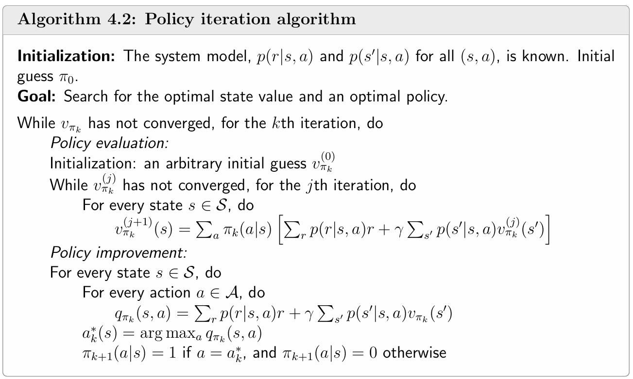

4.3 Truncated policy iteration

We will see that the value iteration and policy iteration algorithms are two special cases of the truncated policy iteration algorithm.

The above steps of the two algorithms can be illustrated as

Policy iteration: $\pi_0 \xrightarrow{P E} v_{\pi_0} \xrightarrow{P I} \pi_1 \xrightarrow{P E} v_{\pi_1} \xrightarrow{P I} \pi_2 \xrightarrow{P E} v_{\pi_2} \xrightarrow{P I} \ldots$.

Value iteration: $\quad \quad \quad v_0 \xrightarrow{P U} \pi_1^{\prime} \xrightarrow{V U} v_1 \xrightarrow{P U} \pi_2^{\prime} \xrightarrow{V U} v_2 \xrightarrow{P U} \ldots$

It can be seen that the procedures of the two algorithms are very similar.
We examine their value steps more closely to see the difference between the two algorithms. In particular, let both algorithms start from the same initial condition: $v_0=v_{\pi_0}$.

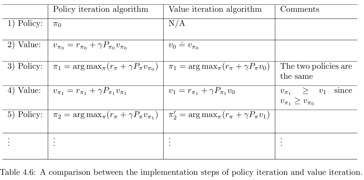
The procedures of the two algorithms are listed in Table 4.6.

• In the first three steps, the two algorithms generate the same results since $v_0=v_{\pi_0}$. They become different in the fourth step.

• During the fourth step, the value iteration algorithm executes $v_1=r_{\pi_1}+\gamma P_{\pi_1} v_0$, which is a one-step calculation , whereas the policy iteration algorithm solves $v_{\pi_1}=r_{\pi_1}+\gamma P_{\pi_1} v_{\pi_1}$, which requires an infinite number of iterations.

If we explicitly write out the iterative process for solving $v_{\pi_1}=r_{\pi_1}+\gamma P_{\pi_1} v_{\pi_1}$ in the fourth step, everything becomes clear. By letting $v_{\pi_1}^{(0)}=v_0$, we have

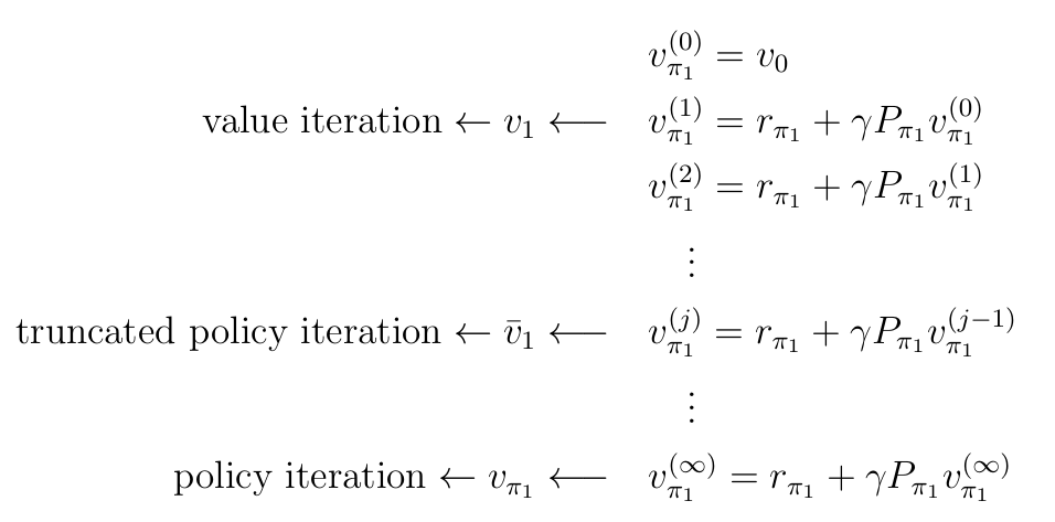
The following observations can be obtained from the above process.

• If the iteration is run only once, then $v_{\pi_1}^{(1)}$ is actually $v_1$, as calculated in the value iteration algorithm.
• iteration is run an infinite number of times, then $v_{\pi_1}^{(\infty)}$ is actually $v_{\pi_1}$, as calculated in the policy iteration algorithm.
• If the iteration is run a finite number of times (denoted as $j_{\text {truncate }}$ ), then such an algorithm is called truncated policy iteration. It is called truncated because the remaining iterations from $j_{\text {truncate }}$ to $\infty$ are truncated.

As a result, the value iteration and policy iteration algorithms can be viewed as two extreme cases of the truncated policy iteration algorithm: value iteration terminates at $j_{\text {truncate }}=1$, and policy iteration terminates at $j_{\text {truncate }}=\infty$.

It should be noted that, although the above comparison is illustrative, it is based on the condition that $v_{\pi_1}^{(0)}=v_0=v_{\pi_0}$. The two algorithms cannot be directly compared without this condition.

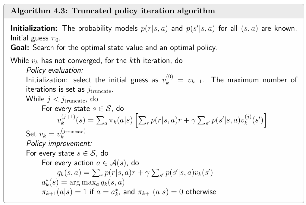
Truncated policy iteration algorithm

In a nutshell, the truncated policy iteration algorithm is the same as the policy iteration algorithm except that it merely runs a finite number of iterations in the policy evaluation step.

Lemma: Value Improvement

Consider the iterative algorithm for solving the policy evaluation step:

$$v_{\pi_k}^{(j+1)}=r_{\pi_k}+\gamma P_{\pi_k} v_{\pi_k}^{(j)}, \quad j=0,1,2, \ldots$$

If the initial guess is selected as $v_{\pi_k}^{(0)}=v_{\pi_{k-1}}$, it holds that

$$v_{\pi_k}^{(j+1)} \geq v_{\pi_k}^{(j)}$$

for every $j=0,1,2, \ldots$.

Proof:
First, since $v_{\pi_k}^{(j)}=r_{\pi_k}+\gamma P_{\pi_k} v_{\pi_k}^{(j-1)}$ and $v_{\pi_k}^{(j+1)}=r_{\pi_k}+\gamma P_{\pi_k} v_{\pi_k}^{(j)}$, we have

$$v_{\pi_k}^{(j+1)}-v_{\pi_k}^{(j)}=\gamma P_{\pi_k}\left(v_{\pi_k}^{(j)}-v_{\pi_k}^{(j-1)}\right)=\cdots=\gamma^j P_{\pi_k}^j\left(v_{\pi_k}^{(1)}-v_{\pi_k}^{(0)}\right)$$

Second, since $v_{\pi_k}^{(0)}=v_{\pi_{k-1}}$, we have

$$v_{\pi_k}^{(1)}=r_{\pi_k}+\gamma P_{\pi_k} v_{\pi_k}^{(0)}=r_{\pi_k}+\gamma P_{\pi_k} v_{\pi_{k-1}} \geq r_{\pi_{k-1}}+\gamma P_{\pi_{k-1}} v_{\pi_{k-1}}=v_{\pi_{k-1}}=v_{\pi_k}^{(0)},$$

where the inequality is due to $\pi_k=\arg \max _\pi\left(r_\pi+\gamma P_\pi v_{\pi_{k-1}}\right)$. Substituting $v_{\pi_k}^{(1)} \geq v_{\pi_k}^{(0)}$ into (4.5) yields $v_{\pi_k}^{(j+1)} \geq v_{\pi_k}^{(j)}$.

Relationships between the three algorithms

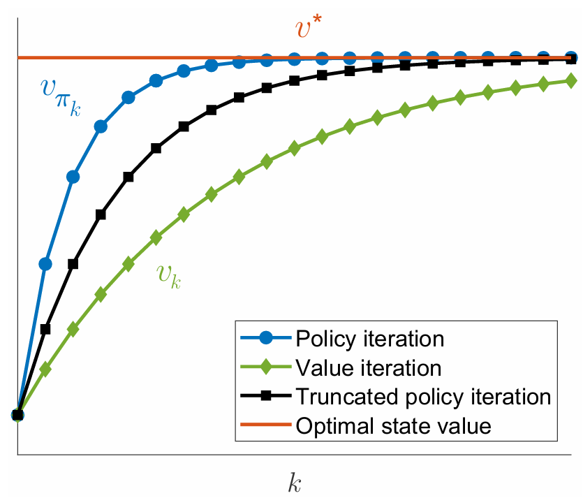
Define $||v_k-v^\ast||$ as the state value error at time $k$. The stop criterion is $||v_k-v^\ast||<0.01$, Truncated policy iteration-$x$.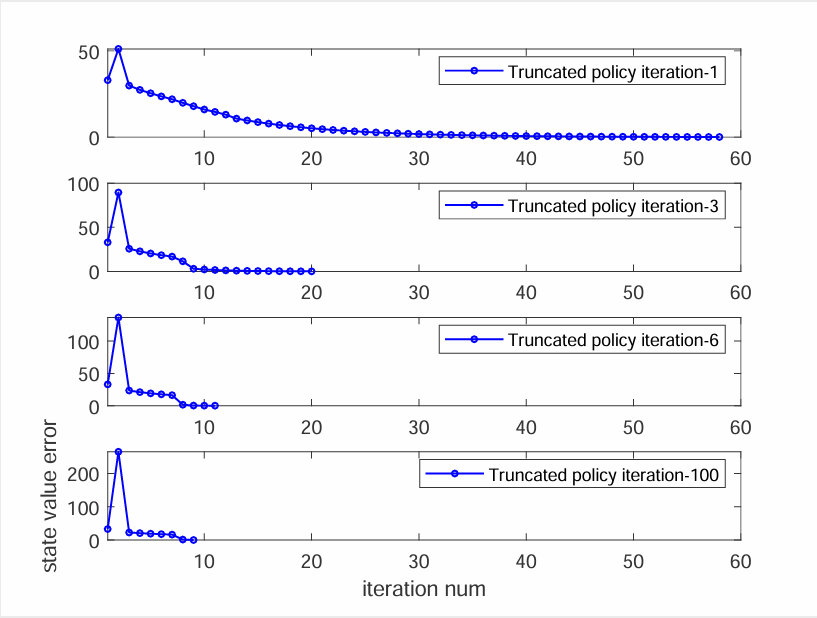

• The greater the value of $x$ is, the faster the value estimate converges.
• However, the benefit of increasing $x$ drops quickly when $x$ is large.
• In practice, run a few number of iterations in the policy evaluation step.

4.4 Summary

• 1 Value iteration: The value iteration algorithm is the same as the algorithm suggested by the contraction mapping theorem for solving the Bellman optimality equation. It can be decomposed into two steps: policy update and value update.

• 2 Policy iteration: The policy iteration algorithm is slightly more complicated than the value iteration algorithm. It also contains two steps: policy evaluation and policy improvement.In the policy evaluation step , an iterative algorithm is required to solve the Bellman equation of the current policy.

• 3 Truncated policy iteration: The value iteration and policy iteration algorithms can be viewed as two extreme cases of the truncated policy iteration algorithm. The intermediate values generated by the truncated policy iteration algorithm are not state values? Only if we run an infinite number of iterations in the policy evaluation step, can we obtain true state values. If we run a nite number of iterations, we can only obtain approximates of the true state values.

A common property of the three algorithms is that every iteration has two steps. One step is to update the value, and the other step is to update the policy. The idea of interaction between value and policy updates widely exists in reinforcement learning algorithms. This idea is also called generalized policy iteration.

Generalized policy iteration is not a specific algorithm. Instead, it refers to the general idea of the interaction between value and policy updates. This idea is rooted in the policy iteration algorithm. Most of the reinforcement learning algorithms introduced in this book fall into the scope of generalized policy iteration.

Finally, the algorithms introduced in this chapter require the system model. Starting in Chapter 5, we will study model-free reinforcement learning algorithms. We will see that the model-free can be obtained by extending the algorithms introduced in this chapter.

Q: What are model-based and model-free reinforcement learning?
A: Although the algorithms introduced in this chapter can find optimal policies, they are usually called dynamic programming algorithms rather than reinforcement learning algorithms because they require the system model. Reinforcement learning algorithms can be classified into two categories: model-based and model-free. Here, model-based does not refer to the requirement of the system model. Instead, model-based reinforcement learning uses data to estimate the system model and uses this model during the learning process. By contrast, model-free reinforcement learning does not involve model estimation during the learning process.

5 Monte Carlo Methods

If we do not have a model, we must have some data. If we do not have data, we must have a model. If we have neither, then we are not able to find optimal policies. The data in reinforcement learning usually refers to the agent’s interaction experiences with the environment.
Model-based reinforcement learning algorithms that need do presume system models.
Model-free reinforcement learning algorithms that do not presume system models.

5.1 Mean estimation problem

we start this chapter by introducing the mean estimation problem, where the expected value of a random variable is estimated from some samples. Understanding this problem is crucial for understanding the fundamental idea of learning from data .
Why we care about the mean estimation problem? It is simply because state and action values are both defined as the means of returns. Estimating a state or action value is actually a mean estimation problem.

Consider a random variable $X$ that can take values from a finite set of real numbers denoted as $\mathcal{X}$, suppose that our task is to calculate the mean or expected value of $X$, i.e., $\mathbb{E}[X]$.

Two approaches can be used to calculate $\mathbb{E}[X]$.

Model based case

The first approach is model-based. Here, the model refers to the probability distribution of $X$. If the model is known, then the mean can be directly calculated based on the definition of the expected value:

$$\mathbb{E}[X]=\sum_{x \in \mathcal{X}} p(x) x$$

Model free case

The second approach is model-free. When the probability distribution (i.e., the model) of $X$ is unknown, suppose that we have some samples $\left\{x_1, x_2, \ldots, x_n\right\}$ of $X$. Then, the mean can be approximated as

$$\mathbb{E}[X] \approx \bar{x}=\frac{1}{n} \sum_{j=1}^n x_j .$$

When $n$ is small, this approximation may not be accurate. However, as $n$ increases, the approximation becomes increasingly accurate. When $n \rightarrow \infty$, we have $\bar{x} \rightarrow \mathbb{E}[X]$.

This is guaranteed by the law of large numbers: the average of a large number of samples is close to the expected value.

It is worth mentioning that the samples used for mean estimation must be independent and identically distributed(i.i.d. or iid). Otherwise, if the sampling values correlate, it may be impossible to correctly estimate the expected value. An extreme case is that all the sampling values are the same as the r st one, whatever the r st one is. In this case, the average of the samples is always equal to the r st sample, no matter how many samples we use.

Law of large numbers
For a random variable $X$, suppose that $\left\{x_i\right\}_{i=1}^n$ are some i.i.d. samples. Let $\bar{x}=$ $\frac{1}{n} \sum_{i=1}^n x_i$ be the average of the samples. Then,

$$\begin{aligned} \mathbb{E}[\bar{x}] & =\mathbb{E}[X], \\ \operatorname{var}[\bar{x}] & =\frac{1}{n} \operatorname{var}[X] . \end{aligned}$$

The above two equations indicate that $\bar{x}$ is an unbiased estimate of $\mathbb{E}[X]$, and its variance decreases to zero as $n$ increases to infinity.
The proof is given below.

First, $\mathbb{E}[\bar{x}]=\mathbb{E}\left[\sum_{i=1}^n x_i / n\right]=\sum_{i=1}^n \mathbb{E}\left[x_i\right] / n=\mathbb{E}[X]$, where the last equability is due to the fact that the samples are identically distributed (that is, $\mathbb{E}\left[x_i\right]=\mathbb{E}[X]$ ).

Second, $\operatorname{var}(\bar{x})=\operatorname{var}\left[\sum_{i=1}^n x_i / n\right]=\sum_{i=1}^n \operatorname{var}\left[x_i\right] / n^2=(n \cdot \operatorname{var}[X]) / n^2=$ $\operatorname{var}[X] / n$, where the second equality is due to the fact that the samples are independent, and the third equability is a result of the samples being identically distributed (that is, $\operatorname{var}\left[x_i\right]=\operatorname{var}[X]$ ).

5.2 MC Basic: The simplest MC-based algorithm

5.2.1 introduction

Recalling that the policy iteration algorithm has two steps in each iteration:

1. Policy evaluation(PE): $v_{\pi_k}=r_{\pi_k}+\gamma P_{\pi_k} v_{\pi_k}$.
2. Policy improvement(PI): $\pi_{k+1}=\arg \max _\pi\left(r_\pi+\gamma P_\pi v_{\pi_k}\right)$.

The PE step is calculated through solving the Bellman equation.

The elementwise form of the (PE,PI) step are:

$$\begin{aligned} v_{\pi_{k}} & =\sum_a \pi(a \mid s)\left[\sum_r p(r \mid s, a) r+\gamma \sum_{s^{\prime}} p\left(s^{\prime} \mid s, a\right) v_{\pi_k}\left(s^{\prime}\right)\right] \\ & =\sum_a \pi(a \mid s) q_{\pi_k}(s, a), \quad s \in \mathcal{S} \end{aligned}$$ $$\begin{aligned} \pi_{k+1}(s) & =\arg \max _\pi \sum_a \pi(a \mid s)\left[\sum_r p(r \mid s, a) r+\gamma \sum_{s^{\prime}} p\left(s^{\prime} \mid s, a\right) v_{\pi_k}\left(s^{\prime}\right)\right] \\ & =\arg \max _\pi \sum_a \pi(a \mid s) q_{\pi_k}(s, a), \quad s \in \mathcal{S} \end{aligned}$$

Under the model free case —— The calculated key is $q_{\pi_k}(s, a)$ ! So how can we calculate $q_{\pi_k}(s, a)$?

Model based case

The policy iteration algorithm is a model based algorithm, the model (or dynamic) is given. a MDP is composed of two parts:

1. State transition probability: $p\left(s^{\prime} \mid s, a\right)$.
2. Reward probability: $p(r \mid s, a)$.

Thus, we can calculate $q_{\pi_k}(s, a)$ via following equation

$$q_{\pi_k}(s, a)=\sum_r p(r \mid s, a) r+\gamma \sum_{s^{\prime}} p\left(s^{\prime} \mid s, a\right) v_{\pi_k}\left(s^{\prime}\right)$$

where $p\left(s^{\prime} \mid s, a\right)$ and $p(r \mid s, a)$ are given, and every $v_{\pi_k}\left(s^{\prime}\right)$ is calculated in the PE step.

Model free case

But what if we don’t know the model, Please recalling the definition of action value.

$$\begin{equation} q_\pi(s, a) \triangleq \mathbb{E}\left[G_t \mid S_t=s, A_t=a\right] \end{equation}$$

We can to calculate $q_{\pi_k}(s, a)$ based on data (samples or experiences). This is the key idea of MCRL: If we don’t have a model, we estimate one based on data (or experience).

The procedure of Monte Carlo estimation of action values

Starting from $(s, a)$, following policy $\pi_k$, generate an episode. The return of this episode is $g(s, a)$. $g(s, a)$ is a sample of $G_t$ in

$$q_{\pi_k}(s, a)=\mathbb{E}\left[G_t \mid S_t=s, A_t=a\right]$$

Suppose we have a set of episodes and hence $\left\{g^{(j)}(s, a)\right\}$. Then,

$$\textcolor{red} {q_{\pi_k}(s, a)=\mathbb{E}\left[G_t \mid S_t=s, A_t=a\right] \approx \frac{1}{N} \sum_{i=1}^N g^{(i)}(s, a)}$$

The idea of estimate the mean based on data is called Monte Carlo estimation. This is why this method is called “MC (Monte Carlo) Basic”.

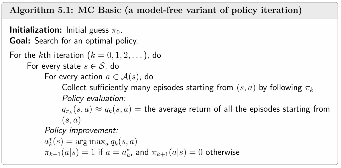
5.2.2 The MC Basic algorithm

The MC Basic algorithm is exactly the same as the policy iteration algorithm except: In policy evaluation (PI), we don’t solve $v_{\pi_k}(s)$, instead we estimate $q_{\pi_k}(s, a)$ directly.

Why we don’t compute $v_{\pi_k}(s)$? Because if we calculate the state value in PE, in PI step we still need to calculate action value. So we can directly calculate action value in PE.

Since policy iteration is convergent, MC Basic is also convergent when given sufficient samples.However, the MC Basic algorithm is not practical due its low sample efficiency (we need to calculate $N$ episodes for every $q_{\pi_k}(s, a)$, it is a large work time ).

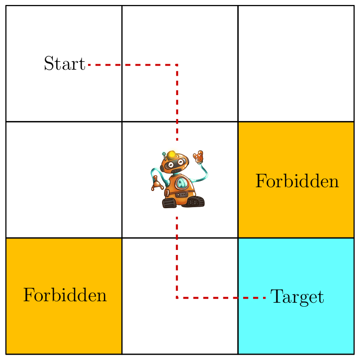
A simple example

An initial policy is shown in the figure (as you can see, it’s a deterministic policy). Use MC Basic to find the optimal policy. The env setting is:

$$r_{\text {boundary }}=-1, r_{\text {forbidden }}=-1, r_{\text {target }}=1, \gamma=0.9 .$$

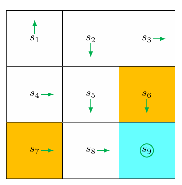
Outline: given the current policy $\pi_k$, in each iteration:

1. policy evaluation: calculate $q_{\pi_k}(s, a)$. Sicne there’re 9 states and 5 actions. We need to calculate 45 state-action pairs.
2. policy improvement: select the greedy action

$$a^*(s)=\arg \max _{a_i} q_{\pi_k}(s, a)$$

For each state-action pair, we need to roll out $N$ episodes to estimate the action value. However, since it’s a deterministic policy, running multiple times would generate the same trajectory. So we only need to rollout a single episode.

For space limitation, we only illustrate for the part of action value for $s_1$ in the first iteration.

Step 1: policy evaluation

1. Starting from $\left(s_1, a_1\right)$, the episode is $s_1 \xrightarrow{a_1} s_1 \xrightarrow{a_1} s_1 \xrightarrow{a_1} \ldots$ Hence, the action value is

$$q_{\pi_0}\left(s_1, a_1\right)=-1+\gamma(-1)+\gamma^2(-1)+\ldots$$

1. Starting from $\left(s_1, a_2\right)$, the episode is $s_1 \xrightarrow{a_2} s_2 \xrightarrow{a_3} s_5 \xrightarrow{a_3} \ldots$ Hence, the action value is

$$q_{\pi_0}\left(s_1, a_2\right)=0+\gamma 0+\gamma^2 0+\gamma^3(1)+\gamma^4(1)+\ldots$$

1. Starting from $\left(s_1, a_3\right)$, the episode is $s_1 \xrightarrow{a_3} s_4 \xrightarrow{a_2} s_5 \xrightarrow{a_3} \ldots$ Hence, the action value is

$$q_{\pi_0}\left(s_1, a_3\right)=0+\gamma 0+\gamma^2 0+\gamma^3(1)+\gamma^4(1)+\ldots$$

1. Starting from $\left(s_1, a_4\right)$, the episode is $s_1 \xrightarrow{a_4} s_1 \xrightarrow{a_1} s_1 \xrightarrow{a_1} \ldots$ Hence, the action value is

$$q_{\pi_0}\left(s_1, a_4\right)=-1+\gamma(-1)+\gamma^2(-1)+\ldots$$

1. Starting from $\left(s_1, a_5\right)$, the episode is $s_1 \xrightarrow{a_5} s_1 \xrightarrow{a_1} s_1 \xrightarrow{a_1} \ldots$ Hence, the action value is

$$q_{\pi_0}\left(s_1, a_5\right)=0+\gamma(-1)+\gamma^2(-1)+\ldots$$

Step2: policy improvement

By observing the action values, we see that $q_{\pi_0}\left(s_1, a_2\right)=q_{\pi_0}\left(s_1, a_3\right)$ are the maximum.

As a result, the policy can be improved as

$$\pi_1\left(a_2 \mid s_1\right)=1 \text { or } \pi_1\left(a_3 \mid s_1\right)=1 \text {. }$$

In either way, the new policy for $s_1$ becomes optimal. In this simple example, the initial policy is already optimal for all the states except $s_1$ and $s_3$. Therefore, the policy can become optimal after merely a single iteration. When the policy is nonoptimal for other states, more iterations are needed.

A comprehensive example: Episode length and sparse rewards

In MC Basic, if the episode length is too short, the algorithm won’t converge. Its convergence comes from the policy iteration algorithm. But if the episode length is too short, each action value won’t be correct, and the premise of the reasoning falls apart.

So how should we know the right length? Isn’t MC Basic too fragile?

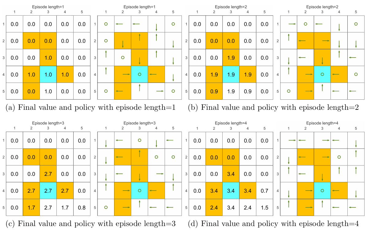
We can see from the following figures that, the episode length greatly impacts the final optimal policies.

When the length of each episode is too short, neither the policy nor the value estimate is optimal (see Figures 5.4(a)-(d)). In the extreme case where the episode length is one, only the states that are adjacent to the target have nonzero values, and all the other states have zero values since each episode is too short to reach the target or get positive rewards (see Figure 5.4(a)).

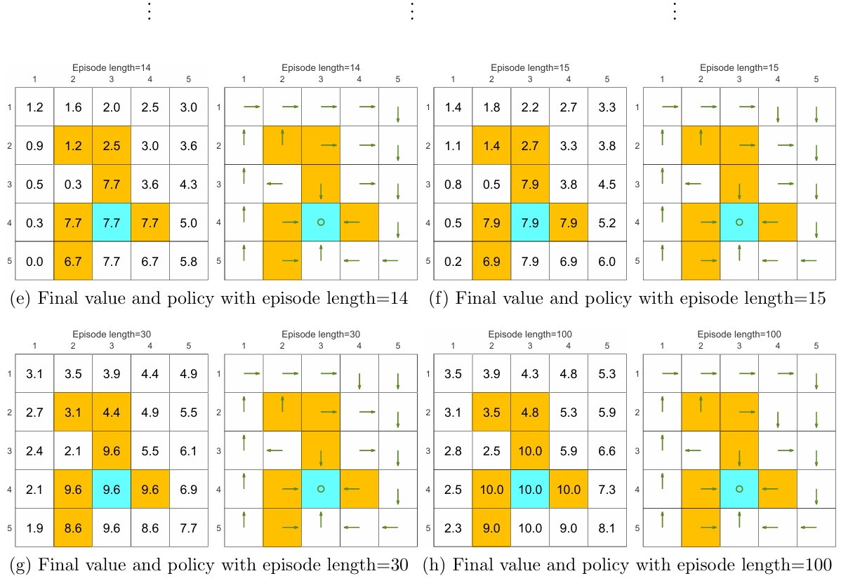
As the episode length increases, the policy and value estimates gradually approach the optimal ones (see Fig- ure 5.4(h)).

While the above analysis suggests that each episode must be sufficiently long, the episodes are not necessarily infinitely long. As shown in Figure 5.4(g), when the length is 30, the algorithm can find an optimal policy, although the value estimate is not yet optimal.

The above analysis is related to an important reward design problem, sparse reward, which refers to the scenario in which no positive rewards can be obtained unless the target is reached. The sparse reward setting requires long episodes that can reach the target. This requirement is challenging to satisfy when the state space is large. As a result, the sparse reward problem downgrades the learning efficiency.

One simple technique for solving this problem is to design nonsparse rewards. For instance, in the above grid world example, we can redesign the reward setting so that the agent can obtain a small positive reward when reaching the states near the target. In this way, an “attractive field” can be formed around the target so that the agent can find the target more easily¹.

¹. M. Riedmiller, R. Hafner, T. Lampe, M. Neunert, J. Degrave, T. Wiele, V. Mnih, N. Heess, and J. T. Springenberg, Learning by playing solving sparse reward tasks from scratch, in International Conference on Machine Learning, pp. 43444353, 2018. ↩

5.3 MC Exploring Starts

5.3.1 Utilizing samples more efficiently

$s_1 \xrightarrow{a_2} s_2 \xrightarrow{a_4} s_1 \xrightarrow{a_2} s_2 \xrightarrow{a_3} s_5 \xrightarrow{a_1}\ldots$

initial visit：an episode is only used to estimate the action value of the initial state-action pair that the episode starts from. The initial-visit strategy merely estimates the action value of $(s_1, a_2)$. The MC Basic algorithm utilizes the initial-visit strategy. However, this strategy is not sample-efficient.because the episode also visits many other state-action pairs such as $(s_2, a_4), (s_2, a_3), (s_5, a_1)$, but they are not be used to estimate the corresponding action values.

subepisode visit：The trajectory generated after the visit of a state-action pair can be viewed as a new episode. In this way, the samples in the episode can be utilized more efficiently.

Moreover, a state-action pair may be visited multiple times in an episode. For example, $(s_1, a_2)$ is visited twice in the below episode. If we only count the first-time visit, this is called a first-visit strategy. If we count every visit of a state-action pair, such a strategy is called every-visit .²

². C. Szepesvari, Algorithms for reinforcement learning. Springer, 2010. ↩

5.3.2 Updating policies more efficiently

The first strategy is, in the policy evaluation step, to collect all the episodes starting from the same state-action pair and then approximate the action value using the average return of these episodes. This strategy is adopted in the MC Basic algorithm. The drawback of this strategy is that the agent must wait until all the episodes have been collected before the estimate can be updated.

The second strategy, which can overcome this drawback, is to use the return of a single episode to approximate the corresponding action value. In this way, we can immediately obtain a rough estimate when we receive an episode. Then, the policy can be improved in an episode-by-episode fashion.(note:this is not step-by-step ,so this is not Temporal-Difference idea)

Since the return of a single episode cannot accurately approximate the corresponding action value, one may wonder whether the second strategy is good. In fact, this strategy falls into the scope of generalized policy iteration introduced in the last chapter. That is, we can still update the policy even if the value estimate is not sufficiently accurate.

5.3.3 Algorithm description

The details of MC Exploring Starts are given in Algorithm 5.2. This algorithm uses the subepisode visit and every-visit strategy. Interestingly, when calculating the discounted return obtained by starting from each state-action pair, the procedure starts from the ending states and travels back to the starting state. Such techniques can make the algorithm more efficient, but it also makes the algorithm more complex.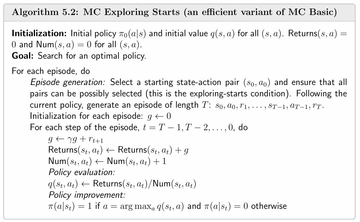

It is worth noting that if an action is not well explored, its action value may be inaccurately estimated, and this action may not be selected by the policy even though it is indeed the best action. Both MC Basic and MC Exploring Starts require this condition. MC Exploring Starts needs to traverse any one $(s, a)$, that is, it needs to start an episode from any one $(s, a)$.

Exploring starts requires an infinite number of (or sufficiently many) episodes to be generated when starting from every state-action pair. In theory, the exploring starts condition is necessary to find optimal policies. That is, only if every action value is well explored, can we accurately evaluate all the actions and then correctly select the optimal ones.

However, this condition is difficult to meet in many applications, especially those involving physical interactions with environments. Can we remove the exploring starts requirement? The answer is yes, as shown in the next section.

5.4 MC $\mathbb{\epsilon}$ -Greedy: Learning without exploring starts

5.4.1 $\mathbb{\epsilon}$-greedy policies

The fundamental idea is to make policies soft. Soft policies are stochastic, enabling an episode to visit many state-action pairs. In this way, we do not need a large number of episodes starting from every state-action pair.

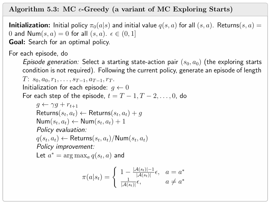
One type of common soft policies is $\mathbb{\epsilon}$-greedy policies. An-greedy policy is a stochastic policy that has a higher chance of choosing the greedy action with the greatest action value. and the same nonzero probability of taking any other action. In particular, suppose that $\mathbb{\epsilon} \in [0,1]$. The corresponding-greedy policy has the following form:

$$\pi_{k+1}(a \mid s)= \begin{cases}1-\frac{\epsilon}{|\mathbb{A}(s)|}(|\mathbb{A}(s)|-1) & \text{for the greedy action} , \\ \frac{\epsilon}{|\mathbb{A}(s)|} & \text{for the other action} |\mathbb{A}(s)|-1 \text{action}.\end{cases} \nonumber$$

• where $|\mathbb{A}(s)|$ denotes the number of actions associated with $s$.
• When $\epsilon= 0$ ,$\epsilon$-greedy becomes greedy. When $\epsilon$= 1, the probability of taking any action equals $\frac{1}{|\mathbb{A}(s)|}$.
• The probability of taking the greedy action is always greater than that of taking any other action because

$$1-\frac{\epsilon}{|\mathbb{A}(s)|}(|\mathbb{A}(s)|-1)=1-\epsilon+\frac{\epsilon}{|\mathbb{A}(s)|} \geq \frac{\epsilon}{|\mathbb{A}(s)|}$$

for any $\mathbb{\epsilon} \in [0,1]$.

5.4.2 Algorithm description

MC $\mathbb{\epsilon}$-Greedy is a variant of MC Exploring Starts that removes the exploring starts requirement.we only need to change the policy improvement step from greedy to $\mathbb{\epsilon}$-greedy.

If greedy policies are replaced by $\epsilon$-greedy policies in the policy improvement step, can we still guarantee to obtain optimal policies?
The answer is both yes and no. By yes, we mean that, when given sufficient samples, the algorithm can converge to an $\mathbb{\epsilon}$-greedy policy that is optimal in the set $\mathbb{\Pi}_{\epsilon}$. By no, we mean that the policy is merely optimal among all-greedy policies $\mathbb{\Pi}_{\epsilon}$ but may not be optimal in $\mathbb{\Pi}$. However, if $\mathbb{\epsilon}$ is sufficiently small, the optimal policies in are close to those in $\mathbb{\Pi}$.

5.4.3 Exploration and exploitation of $\mathbb{\epsilon}$-greedy policies

Exploration and exploitation constitute a fundamental tradeoff in reinforcement learning. Here, exploration means that the policy can possibly take as many actions as possible. In this way, all the actions can be visited and evaluated well. Exploitation means that the improved policy should take the greedy action that has the greatest action value. However, since the action values obtained at the current moment may not be accurate due to insufficient exploration, we should keep exploring while conducting exploitation to avoid missing optimal actions.(exploration-exploitation dilemma,EvE )

$\mathbb{\epsilon}$-greedy policies provide one way to balance exploration and exploitation. If we would like to enhance exploitation and optimality, we need to reduce the value of $\mathbb{\epsilon}$. However, if we would like to enhance exploration, we need to increase the value of $\mathbb{\epsilon}$.

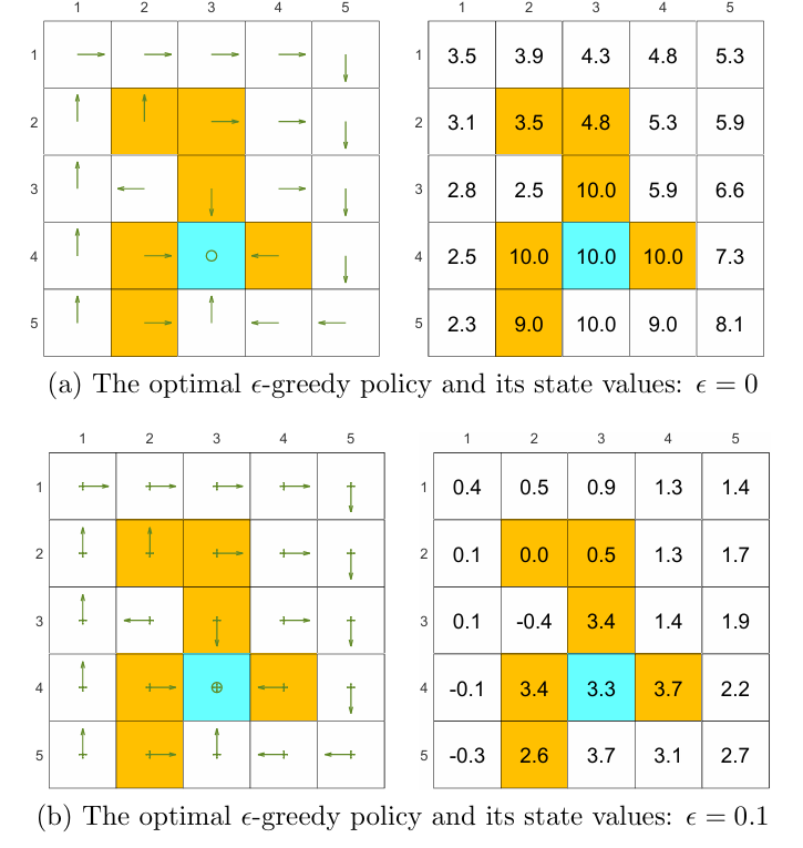
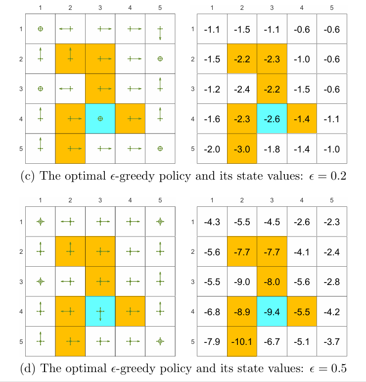
Show in Figure 5.7, as the value of increases, the state values of the-greedy policies decrease, indicating that the optimality of these-greedy policies becomes worse. if we want to obtain-greedy policies that are consistent with the optimal greedy ones, the value of should be sufficiently small.

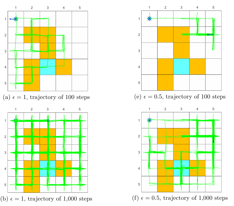
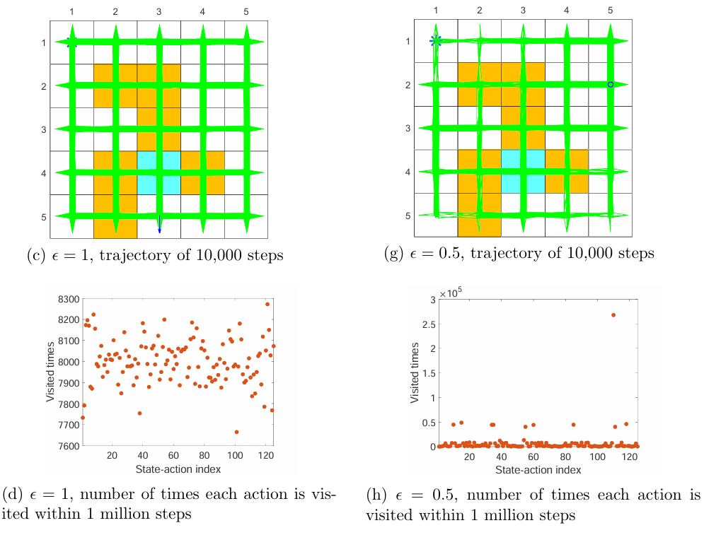
Show in Figure 5.8, it is clear that the exploration ability of an $\mathbb{\epsilon}$-greedy policy is strong when $\mathbb{\epsilon}$ is large.One useful technique is to initially set to be large to enhance exploration and gradually reduce it to ensure the optimality of the final policy ³.

³. A. Maroti, RBED: Reward based epsilon decay, arXiv:1910.13701, 2019. AND Human-level control through deep reinforcement learning, Nature, vol. 518, no. 7540, pp. 529533, 2015 ↩

5.5 Summary

• MC Basic: This is the simplest MC-based reinforcement learning algorithm. This algorithm is obtained by replacing the model-based policy evaluation step in the policy iteration algorithm with a model-free MC-based estimation component. Given sufficient samples, it is guaranteed that this algorithm can converge to optimal policies and optimal state values.

• MC Exploring Starts: This algorithm is a variant of MC Basic. It is a variant of MC Basic that adjusts the sample usage strategy.

• MC-Greedy: This algorithm is a variant of MC Exploring Starts. Specifically, in the policy improvement step, it searches for the best $\mathbb{\epsilon}$-greedy policies instead of greedy policies. In this way, the exploration ability of the policy is enhanced and hence the condition of exploring starts can be removed.

Finally, a tradeoff between exploration and exploitation was introduced by examining the properties of $\mathbb{\epsilon}$-greedy policies.